BGC Sample Project

BGC Sample Project#

In this notebook, the code has the simplest regional ocean model setup possible through CrocoDash. In the comments and descriptions, we’ll provide some of the ways you can add and build on this demo (recreate a specific domain - like GFDL’s NWA12, run with CICE - the sea-ice model in CESM, run with MARBL - the ocean BGC model in CESM, and beyond!)

This notebook is designed for new users of CrocoDash and CESM who want to set up a simple regional ocean model. By following the steps, you will learn how to generate a domain, configure a CESM case, prepare ocean forcing data, and run your simulation.

A typical workflow of utilizing CrocoDash consists of four main steps:

Generate a regional MOM6 domain.
Create the CESM case.
Prepare ocean forcing data.
Build and run the case.

Every specialization of CrocoDash will use this framework.

SECTION 1: Generate a regional MOM6 domain#

We begin by defining a regional MOM6 domain using CrocoDash. To do so, we first generate a horizontal grid. We then generate the topography by remapping an existing bathymetric dataset to our horizontal grid. Finally, we define a vertical grid.

Step 1.1: Horizontal Grid#

from CrocoDash.grid import Grid

grid = Grid(
  resolution=0.1, # in degrees
  xstart=228.0, # min longitude in [0, 360]
  lenx=16.5, # longitude extent in degrees
  ystart=30, # min latitude in [-90, 90]
  leny=20, # latitude extent in degrees
  name="CAcurrent",

# Try changing the grid resolution or domain boundaries to model a different region!

The above cell is a way to generate a rectangular lat/lon grid through CrocoDash

If you’re interested in using an already generated regional grid, you can do that by passing in a supergrid, like in this demo.

If you’re interested in subsetting an already generated global grid, you can do that by passing in lat/lon args, like in this demo.

Step 1.2: Topography#

The below three cells are a way to generate topography with a given grid using the GEBCO dataset.

If you’re interested in using a previously generated topography for your grid, you can do that by passing in a topography file, like in this demo.

from CrocoDash.topo import Topo

topo = Topo(
    grid = grid,
    min_depth = 9.5, # in meters
)

bathymetry_path='/glade/campaign/cgd/oce/projects/CROCODILE/workshops/2025/CrocoDash/data/gebco/GEBCO_2024.nc'

topo.interpolate_from_file(
    file_path = bathymetry_path,
    longitude_coordinate_name="lon",
    latitude_coordinate_name="lat",
    vertical_coordinate_name="elevation"
)

# Validate that the topography looks right!
topo.depth.plot()

Editing the topography#

Regridding topography from GEBCO may result in features we do not necessarily want. The Topo Editor is a tool to edit the bathymetry as wanted. You can do things like erasing basins, opening or closing bays, or adjusting the minimum depth. On JupyterHub, remember we need the ipympl extension, which can be installed as shown on this slide.

topo.depth.plot() before editing

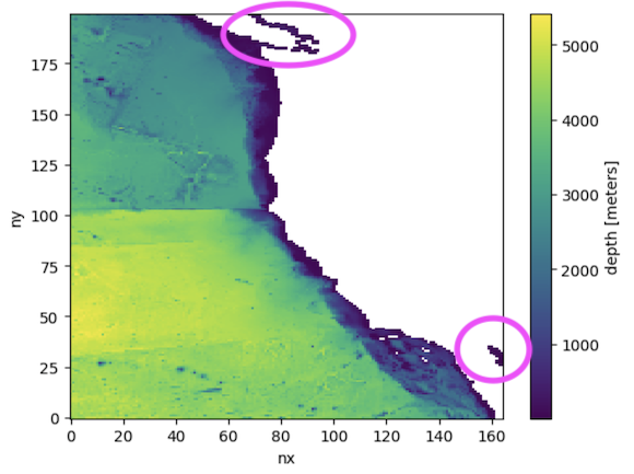
For this particular case, you will need to mask out two disconnected basins (Gulf of California and part of the Salish Sea that gets landlocked at this resolution).

%matplotlib ipympl
from CrocoDash.topo_editor import TopoEditor
TopoEditor(topo)

Step 1.3: Vertical Grid#

The below cell generates a vertical grid using a hyperbolic function. We can also create a uniform grid instance, or use a previously generated vertical grid, like in this demo.

from CrocoDash.vgrid import VGrid

vgrid  = VGrid.hyperbolic(
    nk = 75, # number of vertical levels
    depth = topo.max_depth,
    ratio=20.0 # target ratio of top to bottom layer thicknesses
)

import matplotlib.pyplot as plt
plt.close()
# Create the plot
for depth in vgrid.z:
    plt.axhline(y=depth, linestyle='-')  # Horizontal lines

plt.ylim(max(vgrid.z) + 10, min(vgrid.z) - 10)  # Invert y-axis so deeper values go down
plt.ylabel("Depth")
plt.title("Vertical Grid")
plt.show()

SECTION 2: Create the CESM case#

After generating the MOM6 domain, the next step is to create a CESM case using CrocoDash. This process is straightforward and involves instantiating the CrocoDash Case object. The Case object requires the following inputs:

CESM Source Directory: A local path to a compatible CESM source copy.
Case Name: A unique name for the CESM case.
Input Directory: The directory where all necessary input files will be written.
MOM6 Domain Objects: The horizontal grid, topography, and vertical grid created in the previous section.
Project ID: (Optional) A project ID, if required by the machine.
Compset: The set of models to be used in the Case. Standalone Ocean, Ocean-BGC, Ocean-Seaice, Ocean-Runoff, etc…

Step 2.1: Specify case name and directories:#

Begin by specifying the case name and the necessary directory paths. Ensure the CESM root directory points to your own local copy of CESM. Below is an example setup:

from pathlib import Path

# CESM case (experiment) name
casename = "CACurrent.001"

# CESM source root (Update this path accordingly!!!)
cesmroot ="/path/to/CROCESM"

# Place where all your input files go 
inputdir = Path.home()/"scratch" / "croc_input" / casename
    
# CESM case directory
caseroot = Path.home() / "croc_cases" / casename

Step 2.2: Create the Case#

To create the CESM case, instantiate the Case object as shown below. This will automatically set up the CESM case based on the provided inputs: The cesmroot argument specifies the path to your local CESM source directory. The caseroot argument defines the directory where the case will be created. CrocoDash will handle all necessary namelist modifications and XML changes to align with the MOM6 domain objects generated earlier.

This is where we can change the model setup to what we want:

Interested in BGC? Check out the demo for how to modify this notebook for BGC.
Interested in CICE? Check out the demo for how to modify this notebook for CICE.
Interested in Data Runoff from GLOFAS (or JRA)? Check out the demo for how to modify this notebook for Data Runoff.

from CrocoDash.case import Case

case = Case(
    cesmroot = cesmroot,
    caseroot = caseroot,
    inputdir = inputdir,
    ocn_grid = grid,
    ocn_vgrid = vgrid,
    ocn_topo = topo,
    project = 'CESM0030',
    override = True,
    machine = "derecho",
    compset = "CR1850MARBL_JRA" # Change this as necessary to include whatever models you want. BGC? change MOM6 to MOM6%MARBL-BIO, CICE? Change SICE to CICE, GLOFAS Runoff? Change SROF to DROF%GLOFAS
)

Section 3: Prepare ocean forcing data#

We need to cut out our ocean forcing. The package expects an initial condition and one time-dependent segment per non-land boundary.

In this notebook, we are forcing with the Copernicus Marine “Glorys” reanalysis dataset.

Step 3.1 Configure Initial Conditions and Forcings#

Interested in adding tides? Check out the demo.
Interested in adding chlorophyll? Check out the demo.
Is the GLORYS data access function not working? Check out alternative options in this demo.

Configure Forcings MUST be modified if BGC or Data Runoff are part of the compset (and will throw an error). Check out the demos to see the changes required: BGC Demo, DROF Demo.

case.configure_forcings(
    date_range = ["2000-01-01 00:00:00", "2000-02-01 00:00:00"],
        data_input_path = "/glade/campaign/collections/cmip/CMIP6/CESM-HR/FOSI_BGC/HR/g.e22.TL319_t13.G1850ECOIAF_JRA_HR.4p2z.001/ocn/proc/tseries/month_1",
        product_name = "CESM_OUTPUT",
        marbl_ic_filepath = "/glade/campaign/collections/gdex/data/d651077/cesmdata/inputdata/ocn/mom/tx0.66v1/ecosys_jan_IC_omip_latlon_1x1_180W_c231221.nc",
        boundaries=['south', 'north', 'west'],  # eastern boundary is land-locked!
)

Step 3.3: Process forcing data#

In this final step, we call the process_forcings method of CrocoDash to cut out and interpolate the initial condition as well as all boundaries. CrocoDash also updates MOM6 runtime parameters and CESM xml variables accordingly.

case.process_forcings() # You can turn off specific processing if it's already been processed previously with process_*name* = False. Ex. case.process_forcings(process_chl = False)

Section 4: Build and run the case#

After completing the previous steps, you are ready to build and run your CESM case. Begin by navigating to the case root directory specified during the case creation. Before proceeding, review the user_nl_mom file located in the case directory. This file contains MOM6 parameter settings that were automatically generated by CrocoDash. Carefully examine these parameters and make any necessary adjustments to fine-tune the model for your specific requirements. While CrocoDash aims to provide a solid starting point, further tuning and adjustments are typically necessary to improve the model for your use case.

Once you have reviewed and modified the parameters as needed, you can build and execute the case using the following commands:

qcmd -- ./case.build
./case.submit