Regional Ocean: Basic Region and Surface Field Visualization#
Note: This notebook is meant to be run with the cupid-analysis kernel (see CUPiD Installation). This notebook is often run by default as part of CESM post-processing steps, but you can also run it manually.
Diagnostics and Plotting Resources#
Highly Recommended:#
Xarray Fundamentals - Earth Environmental Data Science Course (recommend the entire course!)
Great! Focused on Global Output Diagnostics#
Misc.#
xGCM - python package for staggered grids
Show code cell source
Hide code cell source
%load_ext autoreload
%autoreload 2
import os

import matplotlib.pyplot as plt
import numpy as np
import regional_utils as utils
import xarray as xr
from cartopy import crs as ccrs
Show code cell source
Hide code cell source
case_name = ""  # "/glade/campaign/cgd/oce/projects/CROCODILE/workshops/2025/Diagnostics/CESM_Output/"
CESM_output_dir = ""  # "CROCODILE_tutorial_nwa12_MARBL"

# As regional domains vary so much in purpose, simulation length, and extent, we don't want to assume a minimum duration
## Thus, we ignore start and end dates and simply reduce/output over the whole time frame for all of the examples given.
start_date = None  # "0001-01-01"
end_date = None  # "0101-01-01

save_figs = False
fig_output_dir = None

lc_kwargs = {}
serial = False

sfc_variables = []  # ['SSH', 'tos', 'sos', 'speed', 'SSV', 'SSU']
monthly_variables = []  # ['thetao', 'so', 'uo', 'vo']
# Parameters
case_name = "CROCODILE_tutorial_nwa12_MARBL"
CESM_output_dir = (
    "/glade/campaign/cgd/oce/projects/CROCODILE/workshops/2025/Diagnostics/CESM_Output/"
)
start_date = ""
end_date = ""
save_figs = True
fig_output_dir = None
lc_kwargs = {"threads_per_worker": 1}
serial = True
sfc_variables = ["tos"]
monthly_variables = ["thetao"]
subset_kwargs = {}
product = "/glade/work/ajanney/crocodile_2025/CUPiD/examples/regional_ocean/computed_notebooks//ocn/Regional_Ocean_Report_Card.ipynb"
Show code cell source
Hide code cell source
OUTDIR = os.path.join(CESM_output_dir, case_name, "ocn", "hist")
print("Output directory is:", OUTDIR)
Output directory is: /glade/campaign/cgd/oce/projects/CROCODILE/workshops/2025/Diagnostics/CESM_Output/CROCODILE_tutorial_nwa12_MARBL/ocn/hist
Load in Model Output and Look at Variables/Meta Data#
Default File Structure in MOM6#
This file structure will be different if you modify the diag_table.
static data: contains horizontal grid, vertical grid, land/sea mask, bathymetry, lat/lon information
sfc data: daily output of 2D surface fields (salinity, temp, SSH, velocities)
monthly data: averaged monthly output of the full 3D domain, regridded to a predefined grid (MOM6 default is WOA, see more below)
native data: averaged monthly output of ocean state and atmospheric fluxes on the native MOM6 grid
Show code cell source
Hide code cell source
# Xarray time decoding things
time_coder = xr.coders.CFDatetimeCoder(use_cftime=True)

## Static data includes hgrid, vgrid, bathymetry, land/sea mask
static_data = xr.open_mfdataset(
    os.path.join(OUTDIR, "*h.static.nc"),
    decode_timedelta=True,
    decode_times=time_coder,
    engine="netcdf4",
)

## Surface Data
sfc_data = xr.open_mfdataset(
    os.path.join(OUTDIR, "*h.sfc*.nc"),
    decode_timedelta=True,
    decode_times=time_coder,
    engine="netcdf4",
)

## Monthly Full Domain Data
## Not used in this notebook by default
monthly_data = xr.open_mfdataset(
    os.path.join(OUTDIR, "*h.z*.nc"),
    decode_timedelta=True,
    decode_times=time_coder,
    engine="netcdf4",
)

## Monthly Full Domain Data, on native MOM6 grid
## Not used in this notebook by default
native_data = xr.open_mfdataset(
    os.path.join(OUTDIR, "*h.native*.nc"),
    decode_timedelta=True,
    decode_times=time_coder,
    engine="netcdf4",
)

## Image/Gif Output Directory
if fig_output_dir is None:
    image_output_dir = os.path.join(
        "/glade/derecho/scratch/",
        os.environ["USER"],
        "archive",
        case_name,
        "ocn",
        "cupid_images",
    )
else:
    image_output_dir = os.path.join(fig_output_dir, case_name, "ocn", "cupid_images")
if not os.path.exists(image_output_dir):
    os.makedirs(image_output_dir)
print("Image output directory is:", image_output_dir)
Image output directory is: /glade/derecho/scratch/ajanney/archive/CROCODILE_tutorial_nwa12_MARBL/ocn/cupid_images
Show code cell source
Hide code cell source
## Select for only the variables we want to analyze
if len(sfc_variables) > 0:
    print("Selecting only the following surface variables:", sfc_variables)
    sfc_data = sfc_data[sfc_variables]
if len(monthly_variables) > 0:
    print("Selecting only the following monthly variables:", monthly_variables)
    monthly_data = monthly_data[monthly_variables]

## Apply time boundaries
## if they are the right format
if len(start_date.split("-")) == 3 and len(end_date.split("-")) == 3:
    import cftime

    calendar = sfc_data.time.encoding.get("calendar", "standard")

    calendar_map = {
        "gregorian": cftime.DatetimeProlepticGregorian,
        "noleap": cftime.DatetimeNoLeap,
    }

    CFTime = calendar_map.get(calendar, cftime.DatetimeGregorian)
    y, m, d = [int(i) for i in start_date.split("-")]
    start_date_time = CFTime(y, m, d)
    y, m, d = [int(i) for i in end_date.split("-")]
    end_date_time = CFTime(y, m, d)

    print(
        f"Applying time range from start_date: {start_date_time} and end_date: {end_date_time}."
    )

    sfc_data = sfc_data.sel(time=slice(start_date_time, end_date_time))
    monthly_data = monthly_data.sel(time=slice(start_date_time, end_date_time))
    native_data = native_data.sel(time=slice(start_date_time, end_date_time))

sfc_time_bounds = [
    sfc_data["time"].isel(time=0).compute().item(),
    sfc_data["time"].isel(time=-1).compute().item(),
]
monthly_time_bounds = [
    monthly_data["time"].isel(time=0).compute().item(),
    monthly_data["time"].isel(time=-1).compute().item(),
]

print(f"Surface Data Time Bounds: {sfc_time_bounds[0]} to {sfc_time_bounds[-1]}")
print(
    f"Monthly Data Time Bounds: {monthly_time_bounds[0]} to {monthly_time_bounds[-1]}"
)
Selecting only the following surface variables: ['tos']
Selecting only the following monthly variables: ['thetao']
Surface Data Time Bounds: 1999-12-30 12:00:00 to 2000-11-28 12:00:00
Monthly Data Time Bounds: 2000-01-14 12:00:00 to 2000-10-14 12:00:00
*mom6.h.static*.nc: static information about the domain#
The MOM6 grid uses an Arakawa C grid which staggers velocities and tracers (temp, salinity, SSH, etc.). See this MOM6 documentation for more information.
Some variables of interest:#
geolon/geolat(and c/u/v variants): specifies the true lat/lon of each cell. We use these variables for plotting and placing the data geographically.wet(and c/u/v variants): the land-sea mask that specifies if a given point is on land or sea.areacello(and bu,cu,cv variants): area of grid cell (important for taking area-weighted averages)deptho: depth of ocean floor - bathymetry
Show code cell source
Hide code cell source
static_data
<xarray.Dataset> Size: 46MB
Dimensions:       (xh: 740, yh: 780, time: 1, xq: 741, yq: 781)
Coordinates:
  * xh            (xh) float64 6kB -97.96 -97.88 -97.79 ... -36.54 -36.46 -36.38
  * yh            (yh) float64 6kB 5.243 5.326 5.409 5.492 ... 53.82 53.86 53.89
  * time          (time) object 8B 0001-01-01 00:00:00
  * xq            (xq) float64 6kB -98.0 -97.92 -97.83 ... -36.5 -36.42 -36.33
  * yq            (yq) float64 6kB 5.201 5.284 5.367 5.45 ... 53.84 53.87 53.91
Data variables: (12/20)
    geolon        (yh, xh) float32 2MB dask.array<chunksize=(780, 740), meta=np.ndarray>
    geolat        (yh, xh) float32 2MB dask.array<chunksize=(780, 740), meta=np.ndarray>
    geolon_c      (yq, xq) float32 2MB dask.array<chunksize=(781, 741), meta=np.ndarray>
    geolat_c      (yq, xq) float32 2MB dask.array<chunksize=(781, 741), meta=np.ndarray>
    geolon_u      (yh, xq) float32 2MB dask.array<chunksize=(780, 741), meta=np.ndarray>
    geolat_u      (yh, xq) float32 2MB dask.array<chunksize=(780, 741), meta=np.ndarray>
    ...            ...
    areacello     (yh, xh) float32 2MB dask.array<chunksize=(780, 740), meta=np.ndarray>
    areacello_cu  (yh, xq) float32 2MB dask.array<chunksize=(780, 741), meta=np.ndarray>
    areacello_cv  (yq, xh) float32 2MB dask.array<chunksize=(781, 740), meta=np.ndarray>
    areacello_bu  (yq, xq) float32 2MB dask.array<chunksize=(781, 741), meta=np.ndarray>
    sin_rot       (yh, xh) float32 2MB dask.array<chunksize=(780, 740), meta=np.ndarray>
    cos_rot       (yh, xh) float32 2MB dask.array<chunksize=(780, 740), meta=np.ndarray>
Attributes:
    NumFilesInSet:  1
    title:          MOM6 diagnostic fields table for CESM case: marbl.bio.croc.5
    grid_type:      regular
grid_tile: N/A- xh: 740
- yh: 780
- time: 1
- xq: 741
- yq: 781
- xh(xh)float64-97.96 -97.88 ... -36.46 -36.38
- units :
- degrees_east
- long_name :
- h point nominal longitude
- axis :
- X
array([-97.958333, -97.875 , -97.791667, ..., -36.541667, -36.458333, -36.375 ], shape=(740,)) - yh(yh)float645.243 5.326 5.409 ... 53.86 53.89
- units :
- degrees_north
- long_name :
- h point nominal latitude
- axis :
- Y
array([ 5.242669, 5.325648, 5.408616, ..., 53.820237, 53.85652 , 53.892753], shape=(780,)) - time(time)object0001-01-01 00:00:00
- long_name :
- time
- axis :
- T
array([cftime.DatetimeGregorian(1, 1, 1, 0, 0, 0, 0, has_year_zero=False)], dtype=object) - xq(xq)float64-98.0 -97.92 ... -36.42 -36.33
- units :
- degrees_east
- long_name :
- q point nominal longitude
- axis :
- X
array([-98. , -97.916667, -97.833333, ..., -36.5 , -36.416667, -36.333333], shape=(741,)) - yq(yq)float645.201 5.284 5.367 ... 53.87 53.91
- units :
- degrees_north
- long_name :
- q point nominal latitude
- axis :
- Y
array([ 5.201175,  5.28416 ,  5.367133, ..., 53.838385, 53.874643, 53.910851],
      shape=(781,))
- geolon(yh, xh)float32dask.array<chunksize=(780, 740), meta=np.ndarray>
- units :
- degrees_east
- long_name :
- Longitude of tracer (T) points
- cell_methods :
- time: point
Array Chunk Bytes 2.20 MiB 2.20 MiB Shape (780, 740) (780, 740) Dask graph 1 chunks in 2 graph layers Data type float32 numpy.ndarray - geolat(yh, xh)float32dask.array<chunksize=(780, 740), meta=np.ndarray>
- units :
- degrees_north
- long_name :
- Latitude of tracer (T) points
- cell_methods :
- time: point
Array Chunk Bytes 2.20 MiB 2.20 MiB Shape (780, 740) (780, 740) Dask graph 1 chunks in 2 graph layers Data type float32 numpy.ndarray - geolon_c(yq, xq)float32dask.array<chunksize=(781, 741), meta=np.ndarray>
- units :
- degrees_east
- long_name :
- Longitude of corner (Bu) points
- cell_methods :
- time: point
- interp_method :
- none
Array Chunk Bytes 2.21 MiB 2.21 MiB Shape (781, 741) (781, 741) Dask graph 1 chunks in 2 graph layers Data type float32 numpy.ndarray - geolat_c(yq, xq)float32dask.array<chunksize=(781, 741), meta=np.ndarray>
- units :
- degrees_north
- long_name :
- Latitude of corner (Bu) points
- cell_methods :
- time: point
- interp_method :
- none
Array Chunk Bytes 2.21 MiB 2.21 MiB Shape (781, 741) (781, 741) Dask graph 1 chunks in 2 graph layers Data type float32 numpy.ndarray - geolon_u(yh, xq)float32dask.array<chunksize=(780, 741), meta=np.ndarray>
- units :
- degrees_east
- long_name :
- Longitude of zonal velocity (Cu) points
- cell_methods :
- time: point
- interp_method :
- none
Array Chunk Bytes 2.20 MiB 2.20 MiB Shape (780, 741) (780, 741) Dask graph 1 chunks in 2 graph layers Data type float32 numpy.ndarray - geolat_u(yh, xq)float32dask.array<chunksize=(780, 741), meta=np.ndarray>
- units :
- degrees_north
- long_name :
- Latitude of zonal velocity (Cu) points
- cell_methods :
- time: point
- interp_method :
- none
Array Chunk Bytes 2.20 MiB 2.20 MiB Shape (780, 741) (780, 741) Dask graph 1 chunks in 2 graph layers Data type float32 numpy.ndarray - geolon_v(yq, xh)float32dask.array<chunksize=(781, 740), meta=np.ndarray>
- units :
- degrees_east
- long_name :
- Longitude of meridional velocity (Cv) points
- cell_methods :
- time: point
- interp_method :
- none
Array Chunk Bytes 2.20 MiB 2.20 MiB Shape (781, 740) (781, 740) Dask graph 1 chunks in 2 graph layers Data type float32 numpy.ndarray - geolat_v(yq, xh)float32dask.array<chunksize=(781, 740), meta=np.ndarray>
- units :
- degrees_north
- long_name :
- Latitude of meridional velocity (Cv) points
- cell_methods :
- time: point
- interp_method :
- none
Array Chunk Bytes 2.20 MiB 2.20 MiB Shape (781, 740) (781, 740) Dask graph 1 chunks in 2 graph layers Data type float32 numpy.ndarray - deptho(yh, xh)float32dask.array<chunksize=(780, 740), meta=np.ndarray>
- units :
- m
- long_name :
- Sea Floor Depth
- cell_methods :
- area:mean yh:mean xh:mean time: point
- cell_measures :
- area: areacello
- standard_name :
- sea_floor_depth_below_geoid
Array Chunk Bytes 2.20 MiB 2.20 MiB Shape (780, 740) (780, 740) Dask graph 1 chunks in 2 graph layers Data type float32 numpy.ndarray - wet(yh, xh)float32dask.array<chunksize=(780, 740), meta=np.ndarray>
- long_name :
- 0 if land, 1 if ocean at tracer points
- cell_methods :
- time: point
- cell_measures :
- area: areacello
Array Chunk Bytes 2.20 MiB 2.20 MiB Shape (780, 740) (780, 740) Dask graph 1 chunks in 2 graph layers Data type float32 numpy.ndarray - wet_c(yq, xq)float32dask.array<chunksize=(781, 741), meta=np.ndarray>
- long_name :
- 0 if land, 1 if ocean at corner (Bu) points
- cell_methods :
- time: point
- interp_method :
- none
Array Chunk Bytes 2.21 MiB 2.21 MiB Shape (781, 741) (781, 741) Dask graph 1 chunks in 2 graph layers Data type float32 numpy.ndarray - wet_u(yh, xq)float32dask.array<chunksize=(780, 741), meta=np.ndarray>
- long_name :
- 0 if land, 1 if ocean at zonal velocity (Cu) points
- cell_methods :
- time: point
- interp_method :
- none
Array Chunk Bytes 2.20 MiB 2.20 MiB Shape (780, 741) (780, 741) Dask graph 1 chunks in 2 graph layers Data type float32 numpy.ndarray - wet_v(yq, xh)float32dask.array<chunksize=(781, 740), meta=np.ndarray>
- long_name :
- 0 if land, 1 if ocean at meridional velocity (Cv) points
- cell_methods :
- time: point
- interp_method :
- none
Array Chunk Bytes 2.20 MiB 2.20 MiB Shape (781, 740) (781, 740) Dask graph 1 chunks in 2 graph layers Data type float32 numpy.ndarray - Coriolis(yq, xq)float32dask.array<chunksize=(781, 741), meta=np.ndarray>
- units :
- s-1
- long_name :
- Coriolis parameter at corner (Bu) points
- cell_methods :
- time: point
- interp_method :
- none
Array Chunk Bytes 2.21 MiB 2.21 MiB Shape (781, 741) (781, 741) Dask graph 1 chunks in 2 graph layers Data type float32 numpy.ndarray - areacello(yh, xh)float32dask.array<chunksize=(780, 740), meta=np.ndarray>
- units :
- m2
- long_name :
- Ocean Grid-Cell Area
- cell_methods :
- area:sum yh:sum xh:sum time: point
- standard_name :
- cell_area
Array Chunk Bytes 2.20 MiB 2.20 MiB Shape (780, 740) (780, 740) Dask graph 1 chunks in 2 graph layers Data type float32 numpy.ndarray - areacello_cu(yh, xq)float32dask.array<chunksize=(780, 741), meta=np.ndarray>
- units :
- m2
- long_name :
- Ocean Grid-Cell Area
- cell_methods :
- area:sum yh:sum xq:sum time: point
- standard_name :
- cell_area
Array Chunk Bytes 2.20 MiB 2.20 MiB Shape (780, 741) (780, 741) Dask graph 1 chunks in 2 graph layers Data type float32 numpy.ndarray - areacello_cv(yq, xh)float32dask.array<chunksize=(781, 740), meta=np.ndarray>
- units :
- m2
- long_name :
- Ocean Grid-Cell Area
- cell_methods :
- area:sum yq:sum xh:sum time: point
- standard_name :
- cell_area
Array Chunk Bytes 2.20 MiB 2.20 MiB Shape (781, 740) (781, 740) Dask graph 1 chunks in 2 graph layers Data type float32 numpy.ndarray - areacello_bu(yq, xq)float32dask.array<chunksize=(781, 741), meta=np.ndarray>
- units :
- m2
- long_name :
- Ocean Grid-Cell Area
- cell_methods :
- area:sum yq:sum xq:sum time: point
- standard_name :
- cell_area
Array Chunk Bytes 2.21 MiB 2.21 MiB Shape (781, 741) (781, 741) Dask graph 1 chunks in 2 graph layers Data type float32 numpy.ndarray - sin_rot(yh, xh)float32dask.array<chunksize=(780, 740), meta=np.ndarray>
- long_name :
- sine of the clockwise angle of the ocean grid north to true north
- cell_methods :
- time: point
Array Chunk Bytes 2.20 MiB 2.20 MiB Shape (780, 740) (780, 740) Dask graph 1 chunks in 2 graph layers Data type float32 numpy.ndarray - cos_rot(yh, xh)float32dask.array<chunksize=(780, 740), meta=np.ndarray>
- long_name :
- cosine of the clockwise angle of the ocean grid north to true north
- cell_methods :
- time: point
Array Chunk Bytes 2.20 MiB 2.20 MiB Shape (780, 740) (780, 740) Dask graph 1 chunks in 2 graph layers Data type float32 numpy.ndarray
- xhPandasIndex
PandasIndex(Index([ -97.95833333333348, -97.875, -97.79166666666674, -97.70833333333348, -97.625, -97.54166666666674, -97.45833333333348, -97.375, -97.29166666666674, -97.20833333333348, ... -37.125, -37.04166666666674, -36.958333333333485, -36.875, -36.79166666666674, -36.708333333333485, -36.625, -36.54166666666674, -36.458333333333485, -36.375], dtype='float64', name='xh', length=740)) - yhPandasIndex
PandasIndex(Index([ 5.242668867430943, 5.325648043338498, 5.408616018163888, 5.491572619468121, 5.574517674931223, 5.657451012353994, 5.740372459659776, 5.823281844896203, 5.906178996236959, 5.989063741983525, ... 53.564822422351234, 53.60146386256571, 53.63805392248538, 53.67459269319862, 53.711080265507746, 53.74751672993067, 53.78390217675452, 53.820236695885875, 53.85652037696807, 53.89275330944369], dtype='float64', name='yh', length=780)) - timePandasIndex
PandasIndex(CFTimeIndex([0001-01-01 00:00:00], dtype='object', length=1, calendar='standard', freq=None)) - xqPandasIndex
PandasIndex(Index([ -98.0, -97.91666666666674, -97.83333333333348, -97.75, -97.66666666666674, -97.58333333333348, -97.5, -97.41666666666674, -97.33333333333348, -97.25, ... -37.083333333333485, -37.0, -36.91666666666674, -36.833333333333485, -36.75, -36.66666666666674, -36.583333333333485, -36.5, -36.41666666666674, -36.333333333333485], dtype='float64', name='xq', length=741)) - yqPandasIndex
PandasIndex(Index([ 5.201175132990646,  5.284159844737953,  5.367133441666669,
        5.450095751278957,  5.533046601195114,  5.615985819155333,
        5.698913233021465,  5.781828670778779,  5.864731960537714,
        5.947622930535634,
       ...
        53.58314957068581,  53.61976530934297,  53.65632971328116,
        53.69284287347758,  53.72930488057105,  53.76571582493504,
       53.802075796656574,  53.83838488558746, 53.874643181222716,
       53.910850772760504],
      dtype='float64', name='yq', length=781))
- NumFilesInSet :
- 1
- title :
- MOM6 diagnostic fields table for CESM case: marbl.bio.croc.5
- grid_type :
- regular
- grid_tile :
- N/A
When accessing the output, we need to pay particular attention to which variables we are accessing and which coordinates correspond to their position on the grid. This also affects plotting and spatial averages (as we will see in this notebook and others).
xh/yh: index the center of the cell inxandyrespectivelyxq/yq: index the corner of the cell inxandyrespectively
Coordinates:
(
xh,yh): center of cell, where tracers are. Plot withgeolon,geolat.(
xh,yq): middle of horizontal interface, where meridional (v) velocity is. Plot withgeolon_v,geolat_v.(
xq,yh): middle of vertical interface, where zonal (u) velocity is. Plot withgeolon_u,geolat_u.(
xq,yq): corners between cells, where vorticity is.
*h.sfc*.nc: daily surface fields#
The surface fields are especially useful for diagnosing short runs. This is not only the most dynamic field for short runs, but it also is the only file that stores daily results (by default). A lot of the diagnostics in this notebook use surface fields because we are able to take time averages and look at time series for any run longer than a couple of days (unlike the full 3D domain fields which are averaged over each month).
Some variables of interest:#
SSH: sea surface heighttos: temperature of ocean surfacesos: salinity of ocean surfacespeed: magnitude of speed (considered a tracer, at the center of a cell)SSUandSSV: zonal and meridional velocity at the surface
Show code cell source
Hide code cell source
sfc_data
<xarray.Dataset> Size: 773MB
Dimensions:  (time: 335, yh: 780, xh: 740)
Coordinates:
  * xh       (xh) float64 6kB -97.96 -97.88 -97.79 ... -36.54 -36.46 -36.38
  * yh       (yh) float64 6kB 5.243 5.326 5.409 5.492 ... 53.82 53.86 53.89
  * time     (time) object 3kB 1999-12-30 12:00:00 ... 2000-11-28 12:00:00
Data variables:
    tos      (time, yh, xh) float32 773MB dask.array<chunksize=(31, 780, 740), meta=np.ndarray>
Attributes:
    NumFilesInSet:     1
    title:             MOM6 diagnostic fields table for CESM case: marbl.bio....
    associated_files:  areacello: marbl.bio.croc.5.mom6.h.static.nc
    grid_type:         regular
grid_tile: N/A- time: 335
- yh: 780
- xh: 740
- xh(xh)float64-97.96 -97.88 ... -36.46 -36.38
- units :
- degrees_east
- long_name :
- h point nominal longitude
- axis :
- X
array([-97.958333, -97.875 , -97.791667, ..., -36.541667, -36.458333, -36.375 ], shape=(740,)) - yh(yh)float645.243 5.326 5.409 ... 53.86 53.89
- units :
- degrees_north
- long_name :
- h point nominal latitude
- axis :
- Y
array([ 5.242669, 5.325648, 5.408616, ..., 53.820237, 53.85652 , 53.892753], shape=(780,)) - time(time)object1999-12-30 12:00:00 ... 2000-11-...
- long_name :
- time
- axis :
- T
- bounds :
- time_bounds
array([cftime.DatetimeGregorian(1999, 12, 30, 12, 0, 0, 0, has_year_zero=False),
       cftime.DatetimeGregorian(1999, 12, 31, 12, 0, 0, 0, has_year_zero=False),
       cftime.DatetimeGregorian(2000, 1, 1, 12, 0, 0, 0, has_year_zero=False),
       ...,
       cftime.DatetimeGregorian(2000, 11, 26, 12, 0, 0, 0, has_year_zero=False),
       cftime.DatetimeGregorian(2000, 11, 27, 12, 0, 0, 0, has_year_zero=False),
       cftime.DatetimeGregorian(2000, 11, 28, 12, 0, 0, 0, has_year_zero=False)],
      shape=(335,), dtype=object)
- tos(time, yh, xh)float32dask.array<chunksize=(31, 780, 740), meta=np.ndarray>
- units :
- degC
- long_name :
- Sea Surface Temperature
- cell_methods :
- area:mean yh:mean xh:mean time: mean
- cell_measures :
- area: areacello
- time_avg_info :
- average_T1,average_T2,average_DT
- standard_name :
- sea_surface_temperature
Array Chunk Bytes 737.62 MiB 68.26 MiB Shape (335, 780, 740) (31, 780, 740) Dask graph 11 chunks in 23 graph layers Data type float32 numpy.ndarray
- xhPandasIndex
PandasIndex(Index([ -97.95833333333348, -97.875, -97.79166666666674, -97.70833333333348, -97.625, -97.54166666666674, -97.45833333333348, -97.375, -97.29166666666674, -97.20833333333348, ... -37.125, -37.04166666666674, -36.958333333333485, -36.875, -36.79166666666674, -36.708333333333485, -36.625, -36.54166666666674, -36.458333333333485, -36.375], dtype='float64', name='xh', length=740)) - yhPandasIndex
PandasIndex(Index([ 5.242668867430943, 5.325648043338498, 5.408616018163888, 5.491572619468121, 5.574517674931223, 5.657451012353994, 5.740372459659776, 5.823281844896203, 5.906178996236959, 5.989063741983525, ... 53.564822422351234, 53.60146386256571, 53.63805392248538, 53.67459269319862, 53.711080265507746, 53.74751672993067, 53.78390217675452, 53.820236695885875, 53.85652037696807, 53.89275330944369], dtype='float64', name='yh', length=780)) - timePandasIndex
PandasIndex(CFTimeIndex([1999-12-30 12:00:00, 1999-12-31 12:00:00, 2000-01-01 12:00:00,
             2000-01-02 12:00:00, 2000-01-03 12:00:00, 2000-01-04 12:00:00,
             2000-01-05 12:00:00, 2000-01-06 12:00:00, 2000-01-07 12:00:00,
             2000-01-08 12:00:00,
             ...
             2000-11-19 12:00:00, 2000-11-20 12:00:00, 2000-11-21 12:00:00,
             2000-11-22 12:00:00, 2000-11-23 12:00:00, 2000-11-24 12:00:00,
             2000-11-25 12:00:00, 2000-11-26 12:00:00, 2000-11-27 12:00:00,
             2000-11-28 12:00:00],
            dtype='object', length=335, calendar='standard', freq='D'))
- NumFilesInSet :
- 1
- title :
- MOM6 diagnostic fields table for CESM case: marbl.bio.croc.5
- associated_files :
- areacello: marbl.bio.croc.5.mom6.h.static.nc
- grid_type :
- regular
- grid_tile :
- N/A
*h.z*.nc: fields for the full 3D domain, averaged monthly, regridded vertically#
These are vertically remapped diagnostics files that capture the full 3D domain, but they only output monthly averages. For runs less than a month, they will average over the full length of the run.
By default, this diagnostics MOM6 regrids output to the vertical grid from the 2009 World Ocean Atlas (35 layers down to 6750 m).
Some variables of interest:#
uoandvo: zonal and meridional velocitythetao: potential temperatureso: salinityvmoandumo: zonal and meridional mass transportvolcello: volume of each cell (important for averaging over a volume of the domain)
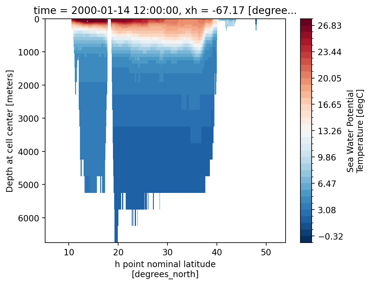
Note: now there are two z coordinates. z_i is the vertical interface between cells and z_l identifies the depth of the cell centers.
Show code cell source
Hide code cell source
monthly_data
<xarray.Dataset> Size: 808MB
Dimensions:  (time: 10, z_l: 35, yh: 780, xh: 740)
Coordinates:
  * yh       (yh) float64 6kB 5.243 5.326 5.409 5.492 ... 53.82 53.86 53.89
  * z_l      (z_l) float64 280B 2.5 10.0 20.0 32.5 ... 5.5e+03 6e+03 6.5e+03
  * time     (time) object 80B 2000-01-14 12:00:00 ... 2000-10-14 12:00:00
  * xh       (xh) float64 6kB -97.96 -97.88 -97.79 ... -36.54 -36.46 -36.38
Data variables:
    thetao   (time, z_l, yh, xh) float32 808MB dask.array<chunksize=(1, 35, 780, 740), meta=np.ndarray>
Attributes:
    NumFilesInSet:     1
    title:             MOM6 diagnostic fields table for CESM case: marbl.bio....
    associated_files:  areacello: marbl.bio.croc.5.mom6.h.static.nc
    grid_type:         regular
grid_tile: N/A- time: 10
- z_l: 35
- yh: 780
- xh: 740
- yh(yh)float645.243 5.326 5.409 ... 53.86 53.89
- units :
- degrees_north
- long_name :
- h point nominal latitude
- axis :
- Y
array([ 5.242669, 5.325648, 5.408616, ..., 53.820237, 53.85652 , 53.892753], shape=(780,)) - z_l(z_l)float642.5 10.0 20.0 ... 6e+03 6.5e+03
- units :
- meters
- long_name :
- Depth at cell center
- axis :
- Z
- positive :
- down
- edges :
- z_i
array([2.5000e+00, 1.0000e+01, 2.0000e+01, 3.2500e+01, 5.1250e+01, 7.5000e+01, 1.0000e+02, 1.2500e+02, 1.5625e+02, 2.0000e+02, 2.5000e+02, 3.1250e+02, 4.0000e+02, 5.0000e+02, 6.0000e+02, 7.0000e+02, 8.0000e+02, 9.0000e+02, 1.0000e+03, 1.1000e+03, 1.2000e+03, 1.3000e+03, 1.4000e+03, 1.5375e+03, 1.7500e+03, 2.0625e+03, 2.5000e+03, 3.0000e+03, 3.5000e+03, 4.0000e+03, 4.5000e+03, 5.0000e+03, 5.5000e+03, 6.0000e+03, 6.5000e+03]) - time(time)object2000-01-14 12:00:00 ... 2000-10-...
- long_name :
- time
- axis :
- T
- bounds :
- time_bounds
array([cftime.DatetimeGregorian(2000, 1, 14, 12, 0, 0, 0, has_year_zero=False), cftime.DatetimeGregorian(2000, 2, 13, 12, 0, 0, 0, has_year_zero=False), cftime.DatetimeGregorian(2000, 3, 14, 12, 0, 0, 0, has_year_zero=False), cftime.DatetimeGregorian(2000, 4, 14, 0, 0, 0, 0, has_year_zero=False), cftime.DatetimeGregorian(2000, 5, 14, 12, 0, 0, 0, has_year_zero=False), cftime.DatetimeGregorian(2000, 6, 14, 0, 0, 0, 0, has_year_zero=False), cftime.DatetimeGregorian(2000, 7, 14, 12, 0, 0, 0, has_year_zero=False), cftime.DatetimeGregorian(2000, 8, 14, 12, 0, 0, 0, has_year_zero=False), cftime.DatetimeGregorian(2000, 9, 14, 0, 0, 0, 0, has_year_zero=False), cftime.DatetimeGregorian(2000, 10, 14, 12, 0, 0, 0, has_year_zero=False)], dtype=object) - xh(xh)float64-97.96 -97.88 ... -36.46 -36.38
- units :
- degrees_east
- long_name :
- h point nominal longitude
- axis :
- X
array([-97.958333, -97.875   , -97.791667, ..., -36.541667, -36.458333,
       -36.375   ], shape=(740,))
- thetao(time, z_l, yh, xh)float32dask.array<chunksize=(1, 35, 780, 740), meta=np.ndarray>
- units :
- degC
- long_name :
- Sea Water Potential Temperature
- cell_methods :
- area:mean z_l:mean yh:mean xh:mean time: mean
- cell_measures :
- volume: volcello area: areacello
- time_avg_info :
- average_T1,average_T2,average_DT
- standard_name :
- sea_water_potential_temperature
Array Chunk Bytes 770.65 MiB 77.06 MiB Shape (10, 35, 780, 740) (1, 35, 780, 740) Dask graph 10 chunks in 21 graph layers Data type float32 numpy.ndarray
- yhPandasIndex
PandasIndex(Index([ 5.242668867430943, 5.325648043338498, 5.408616018163888, 5.491572619468121, 5.574517674931223, 5.657451012353994, 5.740372459659776, 5.823281844896203, 5.906178996236959, 5.989063741983525, ... 53.564822422351234, 53.60146386256571, 53.63805392248538, 53.67459269319862, 53.711080265507746, 53.74751672993067, 53.78390217675452, 53.820236695885875, 53.85652037696807, 53.89275330944369], dtype='float64', name='yh', length=780)) - z_lPandasIndex
PandasIndex(Index([ 2.5, 10.0, 20.0, 32.5, 51.25, 75.0, 100.0, 125.0, 156.25, 200.0, 250.0, 312.5, 400.0, 500.0, 600.0, 700.0, 800.0, 900.0, 1000.0, 1100.0, 1200.0, 1300.0, 1400.0, 1537.5, 1750.0, 2062.5, 2500.0, 3000.0, 3500.0, 4000.0, 4500.0, 5000.0, 5500.0, 6000.0, 6500.0], dtype='float64', name='z_l')) - timePandasIndex
PandasIndex(CFTimeIndex([2000-01-14 12:00:00, 2000-02-13 12:00:00, 2000-03-14 12:00:00, 2000-04-14 00:00:00, 2000-05-14 12:00:00, 2000-06-14 00:00:00, 2000-07-14 12:00:00, 2000-08-14 12:00:00, 2000-09-14 00:00:00, 2000-10-14 12:00:00], dtype='object', length=10, calendar='standard', freq=None)) - xhPandasIndex
PandasIndex(Index([ -97.95833333333348,             -97.875,  -97.79166666666674,
        -97.70833333333348,             -97.625,  -97.54166666666674,
        -97.45833333333348,             -97.375,  -97.29166666666674,
        -97.20833333333348,
       ...
                   -37.125,  -37.04166666666674, -36.958333333333485,
                   -36.875,  -36.79166666666674, -36.708333333333485,
                   -36.625,  -36.54166666666674, -36.458333333333485,
                   -36.375],
      dtype='float64', name='xh', length=740))
- NumFilesInSet :
- 1
- title :
- MOM6 diagnostic fields table for CESM case: marbl.bio.croc.5
- associated_files :
- areacello: marbl.bio.croc.5.mom6.h.static.nc
- grid_type :
- regular
- grid_tile :
- N/A
The output found in *mom6.h.z.*.nc files is vertically remapped by MOM6. By default, this output is on the 2009 World Ocean Atlas grid. You can regrid the output after runtime (see packages like xgcm and and xESMF), but if you know a vertical grid that you need output on, MOM6 can handle the interpolation automatically.
The vertical grid settings for a particular CESM run can be found in MOM_parameter_doc.all in the CESM case run directory. See this MOM6 documentation for more information.
*h.native*.nc: fields for the full 3D domain, averaged monthly, on native MOM6 grid.#
These outputs are on the MOM6 native grid. From the MOM6 Documentation:
Since the model can be run in arbitrary coordinates, say in hybrid-coordinate mode, then native-space diagnostics can be potentially confusing. Native diagnostics are useful when examining exactly what the model is doing
The default native file (as configured by CESM) also outputs useful global averages and atmospheric variables.
Some variables of interest:#
soga: global mean ocean salinitythetaoga: global mean ocean potential temperaturetauuoandtauvo: zonal and meridional downward stress from the atmospheric forcinghfds: net downward surface heat fluxhf*: various individual heat fluxes into the ocean
friver: freshwater flux from rivers
native_data
<xarray.Dataset> Size: 39GB
Dimensions:               (time: 11, scalar_axis: 1, zl: 75, yh: 780, xq: 741,
                           yq: 781, xh: 740, zi: 76, nbnd: 2)
Coordinates:
  * scalar_axis           (scalar_axis) float64 8B 0.0
  * time                  (time) object 88B 2000-01-14 12:00:00 ... 2000-11-1...
  * nbnd                  (nbnd) float64 16B 1.0 2.0
  * xq                    (xq) float64 6kB -98.0 -97.92 -97.83 ... -36.42 -36.33
  * yh                    (yh) float64 6kB 5.243 5.326 5.409 ... 53.86 53.89
  * zl                    (zl) float64 600B 1.0 3.0 5.0 ... 6.125e+03 6.375e+03
  * xh                    (xh) float64 6kB -97.96 -97.88 ... -36.46 -36.38
  * yq                    (yq) float64 6kB 5.201 5.284 5.367 ... 53.87 53.91
  * zi                    (zi) float64 608B 0.0 2.0 4.0 ... 6.25e+03 6.5e+03
Data variables: (12/76)
    soga                  (time, scalar_axis) float32 44B dask.array<chunksize=(1, 1), meta=np.ndarray>
    thetaoga              (time, scalar_axis) float32 44B dask.array<chunksize=(1, 1), meta=np.ndarray>
    uh                    (time, zl, yh, xq) float32 2GB dask.array<chunksize=(1, 75, 780, 741), meta=np.ndarray>
    vh                    (time, zl, yq, xh) float32 2GB dask.array<chunksize=(1, 75, 781, 740), meta=np.ndarray>
    vhbt                  (time, yq, xh) float32 25MB dask.array<chunksize=(1, 781, 740), meta=np.ndarray>
    uhbt                  (time, yh, xq) float32 25MB dask.array<chunksize=(1, 780, 741), meta=np.ndarray>
    ...                    ...
    speed                 (time, yh, xh) float32 25MB dask.array<chunksize=(1, 780, 740), meta=np.ndarray>
    mlotst                (time, yh, xh) float32 25MB dask.array<chunksize=(1, 780, 740), meta=np.ndarray>
    average_T1            (time) object 88B dask.array<chunksize=(1,), meta=np.ndarray>
    average_T2            (time) object 88B dask.array<chunksize=(1,), meta=np.ndarray>
    average_DT            (time) timedelta64[ns] 88B dask.array<chunksize=(1,), meta=np.ndarray>
    time_bounds           (time, nbnd) object 176B dask.array<chunksize=(1, 2), meta=np.ndarray>
Attributes:
    NumFilesInSet:     1
    title:             MOM6 diagnostic fields table for CESM case: marbl.bio....
    associated_files:  areacello: marbl.bio.croc.5.mom6.h.static.nc
    grid_type:         regular
grid_tile: N/A- time: 11
- scalar_axis: 1
- zl: 75
- yh: 780
- xq: 741
- yq: 781
- xh: 740
- zi: 76
- nbnd: 2
- scalar_axis(scalar_axis)float640.0
- long_name :
- none
array([0.])
- time(time)object2000-01-14 12:00:00 ... 2000-11-...
- long_name :
- time
- axis :
- T
- bounds :
- time_bounds
array([cftime.DatetimeGregorian(2000, 1, 14, 12, 0, 0, 0, has_year_zero=False), cftime.DatetimeGregorian(2000, 2, 13, 12, 0, 0, 0, has_year_zero=False), cftime.DatetimeGregorian(2000, 3, 14, 12, 0, 0, 0, has_year_zero=False), cftime.DatetimeGregorian(2000, 4, 14, 0, 0, 0, 0, has_year_zero=False), cftime.DatetimeGregorian(2000, 5, 14, 12, 0, 0, 0, has_year_zero=False), cftime.DatetimeGregorian(2000, 6, 14, 0, 0, 0, 0, has_year_zero=False), cftime.DatetimeGregorian(2000, 7, 14, 12, 0, 0, 0, has_year_zero=False), cftime.DatetimeGregorian(2000, 8, 14, 12, 0, 0, 0, has_year_zero=False), cftime.DatetimeGregorian(2000, 9, 14, 0, 0, 0, 0, has_year_zero=False), cftime.DatetimeGregorian(2000, 10, 14, 12, 0, 0, 0, has_year_zero=False), cftime.DatetimeGregorian(2000, 11, 14, 0, 0, 0, 0, has_year_zero=False)], dtype=object) - nbnd(nbnd)float641.0 2.0
- long_name :
- bounds
array([1., 2.])
- xq(xq)float64-98.0 -97.92 ... -36.42 -36.33
- units :
- degrees_east
- long_name :
- q point nominal longitude
- axis :
- X
array([-98. , -97.916667, -97.833333, ..., -36.5 , -36.416667, -36.333333], shape=(741,)) - yh(yh)float645.243 5.326 5.409 ... 53.86 53.89
- units :
- degrees_north
- long_name :
- h point nominal latitude
- axis :
- Y
array([ 5.242669, 5.325648, 5.408616, ..., 53.820237, 53.85652 , 53.892753], shape=(780,)) - zl(zl)float641.0 3.0 5.0 ... 6.125e+03 6.375e+03
- units :
- meter
- long_name :
- Layer pseudo-depth, -z*
- axis :
- Z
- positive :
- down
array([1.000000e+00, 3.000000e+00, 5.000000e+00, 7.000000e+00, 9.005000e+00, 1.101500e+01, 1.303000e+01, 1.505500e+01, 1.709500e+01, 1.916000e+01, 2.125500e+01, 2.338500e+01, 2.556000e+01, 2.779500e+01, 3.010000e+01, 3.249000e+01, 3.498500e+01, 3.760500e+01, 4.037500e+01, 4.332000e+01, 4.647500e+01, 4.988000e+01, 5.357500e+01, 5.761000e+01, 6.205000e+01, 6.697000e+01, 7.245500e+01, 7.861000e+01, 8.555500e+01, 9.342500e+01, 1.023850e+02, 1.126300e+02, 1.243850e+02, 1.379100e+02, 1.535100e+02, 1.715350e+02, 1.923800e+02, 2.164950e+02, 2.443850e+02, 2.766050e+02, 3.137650e+02, 3.565200e+02, 4.055650e+02, 4.616300e+02, 5.254550e+02, 5.977700e+02, 6.792850e+02, 7.706650e+02, 8.725000e+02, 9.852750e+02, 1.109355e+03, 1.244970e+03, 1.392185e+03, 1.550895e+03, 1.720835e+03, 1.901575e+03, 2.092530e+03, 2.292985e+03, 2.502125e+03, 2.719060e+03, 2.942855e+03, 3.172565e+03, 3.407260e+03, 3.646055e+03, 3.888130e+03, 4.132750e+03, 4.379275e+03, 4.627165e+03, 4.875980e+03, 5.125380e+03, 5.375120e+03, 5.625030e+03, 5.875005e+03, 6.125000e+03, 6.375000e+03]) - xh(xh)float64-97.96 -97.88 ... -36.46 -36.38
- units :
- degrees_east
- long_name :
- h point nominal longitude
- axis :
- X
array([-97.958333, -97.875 , -97.791667, ..., -36.541667, -36.458333, -36.375 ], shape=(740,)) - yq(yq)float645.201 5.284 5.367 ... 53.87 53.91
- units :
- degrees_north
- long_name :
- q point nominal latitude
- axis :
- Y
array([ 5.201175, 5.28416 , 5.367133, ..., 53.838385, 53.874643, 53.910851], shape=(781,)) - zi(zi)float640.0 2.0 4.0 ... 6.25e+03 6.5e+03
- units :
- meter
- long_name :
- Interface pseudo-depth, -z*
- axis :
- Z
- positive :
- down
array([0.00000e+00, 2.00000e+00, 4.00000e+00, 6.00000e+00, 8.00000e+00,
       1.00100e+01, 1.20200e+01, 1.40400e+01, 1.60700e+01, 1.81200e+01,
       2.02000e+01, 2.23100e+01, 2.44600e+01, 2.66600e+01, 2.89300e+01,
       3.12700e+01, 3.37100e+01, 3.62600e+01, 3.89500e+01, 4.18000e+01,
       4.48400e+01, 4.81100e+01, 5.16500e+01, 5.55000e+01, 5.97200e+01,
       6.43800e+01, 6.95600e+01, 7.53500e+01, 8.18700e+01, 8.92400e+01,
       9.76100e+01, 1.07160e+02, 1.18100e+02, 1.30670e+02, 1.45150e+02,
       1.61870e+02, 1.81200e+02, 2.03560e+02, 2.29430e+02, 2.59340e+02,
       2.93870e+02, 3.33660e+02, 3.79380e+02, 4.31750e+02, 4.91510e+02,
       5.59400e+02, 6.36140e+02, 7.22430e+02, 8.18900e+02, 9.26100e+02,
       1.04445e+03, 1.17426e+03, 1.31568e+03, 1.46869e+03, 1.63310e+03,
       1.80857e+03, 1.99458e+03, 2.19048e+03, 2.39549e+03, 2.60876e+03,
       2.82936e+03, 3.05635e+03, 3.28878e+03, 3.52574e+03, 3.76637e+03,
       4.00989e+03, 4.25561e+03, 4.50294e+03, 4.75139e+03, 5.00057e+03,
       5.25019e+03, 5.50005e+03, 5.75001e+03, 6.00000e+03, 6.25000e+03,
       6.50000e+03])
- soga(time, scalar_axis)float32dask.array<chunksize=(1, 1), meta=np.ndarray>
- units :
- psu
- long_name :
- Global Mean Ocean Salinity
- cell_methods :
- time: mean
- time_avg_info :
- average_T1,average_T2,average_DT
- standard_name :
- sea_water_salinity
Array Chunk Bytes 44 B 4 B Shape (11, 1) (1, 1) Dask graph 11 chunks in 23 graph layers Data type float32 numpy.ndarray - thetaoga(time, scalar_axis)float32dask.array<chunksize=(1, 1), meta=np.ndarray>
- units :
- degC
- long_name :
- Global Mean Ocean Potential Temperature
- cell_methods :
- time: mean
- time_avg_info :
- average_T1,average_T2,average_DT
- standard_name :
- sea_water_potential_temperature
Array Chunk Bytes 44 B 4 B Shape (11, 1) (1, 1) Dask graph 11 chunks in 23 graph layers Data type float32 numpy.ndarray - uh(time, zl, yh, xq)float32dask.array<chunksize=(1, 75, 780, 741), meta=np.ndarray>
- units :
- m3 s-1
- long_name :
- Zonal Thickness Flux
- cell_methods :
- zl:sum yh:sum xq:point time: mean
- time_avg_info :
- average_T1,average_T2,average_DT
- interp_method :
- none
Array Chunk Bytes 1.78 GiB 165.36 MiB Shape (11, 75, 780, 741) (1, 75, 780, 741) Dask graph 11 chunks in 23 graph layers Data type float32 numpy.ndarray - vh(time, zl, yq, xh)float32dask.array<chunksize=(1, 75, 781, 740), meta=np.ndarray>
- units :
- m3 s-1
- long_name :
- Meridional Thickness Flux
- cell_methods :
- zl:sum yq:point xh:sum time: mean
- time_avg_info :
- average_T1,average_T2,average_DT
- interp_method :
- none
Array Chunk Bytes 1.78 GiB 165.35 MiB Shape (11, 75, 781, 740) (1, 75, 781, 740) Dask graph 11 chunks in 23 graph layers Data type float32 numpy.ndarray - vhbt(time, yq, xh)float32dask.array<chunksize=(1, 781, 740), meta=np.ndarray>
- units :
- m3 s-1
- long_name :
- Barotropic meridional transport averaged over a baroclinic step
- cell_methods :
- yq:point xh:mean time: mean
- time_avg_info :
- average_T1,average_T2,average_DT
- interp_method :
- none
Array Chunk Bytes 24.25 MiB 2.20 MiB Shape (11, 781, 740) (1, 781, 740) Dask graph 11 chunks in 23 graph layers Data type float32 numpy.ndarray - uhbt(time, yh, xq)float32dask.array<chunksize=(1, 780, 741), meta=np.ndarray>
- units :
- m3 s-1
- long_name :
- Barotropic zonal transport averaged over a baroclinic step
- cell_methods :
- yh:mean xq:point time: mean
- time_avg_info :
- average_T1,average_T2,average_DT
- interp_method :
- none
Array Chunk Bytes 24.25 MiB 2.20 MiB Shape (11, 780, 741) (1, 780, 741) Dask graph 11 chunks in 23 graph layers Data type float32 numpy.ndarray - T_ady_2d(time, yq, xh)float32dask.array<chunksize=(1, 781, 740), meta=np.ndarray>
- units :
- W
- long_name :
- Vertically Integrated Advective Meridional Flux of Heat
- cell_methods :
- yq:point xh:sum time: mean
- time_avg_info :
- average_T1,average_T2,average_DT
- interp_method :
- none
Array Chunk Bytes 24.25 MiB 2.20 MiB Shape (11, 781, 740) (1, 781, 740) Dask graph 11 chunks in 23 graph layers Data type float32 numpy.ndarray - T_adx_2d(time, yh, xq)float32dask.array<chunksize=(1, 780, 741), meta=np.ndarray>
- units :
- W
- long_name :
- Vertically Integrated Advective Zonal Flux of Heat
- cell_methods :
- yh:sum xq:point time: mean
- time_avg_info :
- average_T1,average_T2,average_DT
- interp_method :
- none
Array Chunk Bytes 24.25 MiB 2.20 MiB Shape (11, 780, 741) (1, 780, 741) Dask graph 11 chunks in 23 graph layers Data type float32 numpy.ndarray - T_diffy_2d(time, yq, xh)float32dask.array<chunksize=(1, 781, 740), meta=np.ndarray>
- units :
- W
- long_name :
- Vertically Integrated Diffusive Meridional Flux of Heat
- cell_methods :
- yq:point xh:sum time: mean
- time_avg_info :
- average_T1,average_T2,average_DT
- interp_method :
- none
Array Chunk Bytes 24.25 MiB 2.20 MiB Shape (11, 781, 740) (1, 781, 740) Dask graph 11 chunks in 23 graph layers Data type float32 numpy.ndarray - T_diffx_2d(time, yh, xq)float32dask.array<chunksize=(1, 780, 741), meta=np.ndarray>
- units :
- W
- long_name :
- Vertically Integrated Diffusive Zonal Flux of Heat
- cell_methods :
- yh:sum xq:point time: mean
- time_avg_info :
- average_T1,average_T2,average_DT
- interp_method :
- none
Array Chunk Bytes 24.25 MiB 2.20 MiB Shape (11, 780, 741) (1, 780, 741) Dask graph 11 chunks in 23 graph layers Data type float32 numpy.ndarray - T_hbd_diffx_2d(time, yh, xq)float32dask.array<chunksize=(1, 780, 741), meta=np.ndarray>
- units :
- W
- long_name :
- Vertically-integrated zonal diffusive flux from the horizontal boundary diffusion scheme for Heat
- cell_methods :
- yh:sum xq:point time: mean
- time_avg_info :
- average_T1,average_T2,average_DT
- interp_method :
- none
Array Chunk Bytes 24.25 MiB 2.20 MiB Shape (11, 780, 741) (1, 780, 741) Dask graph 11 chunks in 23 graph layers Data type float32 numpy.ndarray - T_hbd_diffy_2d(time, yq, xh)float32dask.array<chunksize=(1, 781, 740), meta=np.ndarray>
- units :
- W
- long_name :
- Vertically-integrated meridional diffusive flux from the horizontal boundary diffusion scheme for Heat
- cell_methods :
- yq:point xh:sum time: mean
- time_avg_info :
- average_T1,average_T2,average_DT
- interp_method :
- none
Array Chunk Bytes 24.25 MiB 2.20 MiB Shape (11, 781, 740) (1, 781, 740) Dask graph 11 chunks in 23 graph layers Data type float32 numpy.ndarray - diftrelo(time, zi, yh, xh)float32dask.array<chunksize=(1, 76, 780, 740), meta=np.ndarray>
- units :
- m2 s-1
- long_name :
- Ocean Tracer Epineutral Laplacian Diffusivity
- cell_methods :
- area:mean zi:point yh:mean xh:mean time: mean
- cell_measures :
- area: areacello
- time_avg_info :
- average_T1,average_T2,average_DT
- standard_name :
- ocean_tracer_epineutral_laplacian_diffusivity
Array Chunk Bytes 1.80 GiB 167.34 MiB Shape (11, 76, 780, 740) (1, 76, 780, 740) Dask graph 11 chunks in 23 graph layers Data type float32 numpy.ndarray - diftrblo(time, zl, yh, xh)float32dask.array<chunksize=(1, 75, 780, 740), meta=np.ndarray>
- units :
- m2 s-1
- long_name :
- Ocean Tracer Diffusivity due to Parameterized Mesoscale Advection
- cell_methods :
- area:mean zl:mean yh:mean xh:mean time: mean
- cell_measures :
- volume: volcello area: areacello
- time_avg_info :
- average_T1,average_T2,average_DT
- standard_name :
- ocean_tracer_diffusivity_due_to_parameterized_mesoscale_advection
Array Chunk Bytes 1.77 GiB 165.14 MiB Shape (11, 75, 780, 740) (1, 75, 780, 740) Dask graph 11 chunks in 23 graph layers Data type float32 numpy.ndarray - difmxybo(time, zl, yh, xh)float32dask.array<chunksize=(1, 75, 780, 740), meta=np.ndarray>
- units :
- m4 s-1
- long_name :
- Ocean lateral biharmonic viscosity
- cell_methods :
- area:mean zl:mean yh:mean xh:mean time: mean
- cell_measures :
- volume: volcello area: areacello
- time_avg_info :
- average_T1,average_T2,average_DT
- standard_name :
- ocean_momentum_xy_biharmonic_diffusivity
Array Chunk Bytes 1.77 GiB 165.14 MiB Shape (11, 75, 780, 740) (1, 75, 780, 740) Dask graph 11 chunks in 23 graph layers Data type float32 numpy.ndarray - volcello(time, zl, yh, xh)float32dask.array<chunksize=(1, 75, 780, 740), meta=np.ndarray>
- units :
- m3
- long_name :
- Ocean grid-cell volume
- cell_methods :
- area:sum zl:sum yh:sum xh:sum time: mean
- time_avg_info :
- average_T1,average_T2,average_DT
- standard_name :
- ocean_volume
Array Chunk Bytes 1.77 GiB 165.14 MiB Shape (11, 75, 780, 740) (1, 75, 780, 740) Dask graph 11 chunks in 23 graph layers Data type float32 numpy.ndarray - vmo(time, zl, yq, xh)float32dask.array<chunksize=(1, 75, 781, 740), meta=np.ndarray>
- units :
- kg s-1
- long_name :
- Ocean Mass Y Transport
- cell_methods :
- zl:sum yq:point xh:sum time: mean
- time_avg_info :
- average_T1,average_T2,average_DT
- standard_name :
- ocean_mass_y_transport
- interp_method :
- none
Array Chunk Bytes 1.78 GiB 165.35 MiB Shape (11, 75, 781, 740) (1, 75, 781, 740) Dask graph 11 chunks in 23 graph layers Data type float32 numpy.ndarray - vhGM(time, zl, yq, xh)float32dask.array<chunksize=(1, 75, 781, 740), meta=np.ndarray>
- units :
- kg s-1
- long_name :
- Time Mean Diffusive Meridional Thickness Flux
- cell_methods :
- zl:sum yq:point xh:sum time: mean
- time_avg_info :
- average_T1,average_T2,average_DT
- interp_method :
- none
Array Chunk Bytes 1.78 GiB 165.35 MiB Shape (11, 75, 781, 740) (1, 75, 781, 740) Dask graph 11 chunks in 23 graph layers Data type float32 numpy.ndarray - vhml(time, zl, yq, xh)float32dask.array<chunksize=(1, 75, 781, 740), meta=np.ndarray>
- units :
- kg s-1
- long_name :
- Meridional Thickness Flux to Restratify Mixed Layer
- cell_methods :
- zl:sum yq:point xh:sum time: mean
- time_avg_info :
- average_T1,average_T2,average_DT
- interp_method :
- none
Array Chunk Bytes 1.78 GiB 165.35 MiB Shape (11, 75, 781, 740) (1, 75, 781, 740) Dask graph 11 chunks in 23 graph layers Data type float32 numpy.ndarray - umo(time, zl, yh, xq)float32dask.array<chunksize=(1, 75, 780, 741), meta=np.ndarray>
- units :
- kg s-1
- long_name :
- Ocean Mass X Transport
- cell_methods :
- zl:sum yh:sum xq:point time: mean
- time_avg_info :
- average_T1,average_T2,average_DT
- standard_name :
- ocean_mass_x_transport
- interp_method :
- none
Array Chunk Bytes 1.78 GiB 165.36 MiB Shape (11, 75, 780, 741) (1, 75, 780, 741) Dask graph 11 chunks in 23 graph layers Data type float32 numpy.ndarray - uhGM(time, zl, yh, xq)float32dask.array<chunksize=(1, 75, 780, 741), meta=np.ndarray>
- units :
- kg s-1
- long_name :
- Time Mean Diffusive Zonal Thickness Flux
- cell_methods :
- zl:sum yh:sum xq:point time: mean
- time_avg_info :
- average_T1,average_T2,average_DT
- interp_method :
- none
Array Chunk Bytes 1.78 GiB 165.36 MiB Shape (11, 75, 780, 741) (1, 75, 780, 741) Dask graph 11 chunks in 23 graph layers Data type float32 numpy.ndarray - uhml(time, zl, yh, xq)float32dask.array<chunksize=(1, 75, 780, 741), meta=np.ndarray>
- units :
- kg s-1
- long_name :
- Zonal Thickness Flux to Restratify Mixed Layer
- cell_methods :
- zl:sum yh:sum xq:point time: mean
- time_avg_info :
- average_T1,average_T2,average_DT
- interp_method :
- none
Array Chunk Bytes 1.78 GiB 165.36 MiB Shape (11, 75, 780, 741) (1, 75, 780, 741) Dask graph 11 chunks in 23 graph layers Data type float32 numpy.ndarray - uo(time, zl, yh, xq)float32dask.array<chunksize=(1, 75, 780, 741), meta=np.ndarray>
- units :
- m s-1
- long_name :
- Sea Water X Velocity
- cell_methods :
- zl:mean yh:mean xq:point time: mean
- time_avg_info :
- average_T1,average_T2,average_DT
- standard_name :
- sea_water_x_velocity
- interp_method :
- none
Array Chunk Bytes 1.78 GiB 165.36 MiB Shape (11, 75, 780, 741) (1, 75, 780, 741) Dask graph 11 chunks in 23 graph layers Data type float32 numpy.ndarray - vo(time, zl, yq, xh)float32dask.array<chunksize=(1, 75, 781, 740), meta=np.ndarray>
- units :
- m s-1
- long_name :
- Sea Water Y Velocity
- cell_methods :
- zl:mean yq:point xh:mean time: mean
- time_avg_info :
- average_T1,average_T2,average_DT
- standard_name :
- sea_water_y_velocity
- interp_method :
- none
Array Chunk Bytes 1.78 GiB 165.35 MiB Shape (11, 75, 781, 740) (1, 75, 781, 740) Dask graph 11 chunks in 23 graph layers Data type float32 numpy.ndarray - h(time, zl, yh, xh)float32dask.array<chunksize=(1, 75, 780, 740), meta=np.ndarray>
- units :
- m
- long_name :
- Layer Thickness
- cell_methods :
- area:mean zl:sum yh:mean xh:mean time: mean
- cell_measures :
- volume: volcello area: areacello
- time_avg_info :
- average_T1,average_T2,average_DT
Array Chunk Bytes 1.77 GiB 165.14 MiB Shape (11, 75, 780, 740) (1, 75, 780, 740) Dask graph 11 chunks in 23 graph layers Data type float32 numpy.ndarray - e(time, zi, yh, xh)float32dask.array<chunksize=(1, 76, 780, 740), meta=np.ndarray>
- units :
- m
- long_name :
- Interface Height Relative to Mean Sea Level
- cell_methods :
- area:mean zi:point yh:mean xh:mean time: mean
- cell_measures :
- area: areacello
- time_avg_info :
- average_T1,average_T2,average_DT
Array Chunk Bytes 1.80 GiB 167.34 MiB Shape (11, 76, 780, 740) (1, 76, 780, 740) Dask graph 11 chunks in 23 graph layers Data type float32 numpy.ndarray - thetao(time, zl, yh, xh)float32dask.array<chunksize=(1, 75, 780, 740), meta=np.ndarray>
- units :
- degC
- long_name :
- Sea Water Potential Temperature
- cell_methods :
- area:mean zl:mean yh:mean xh:mean time: mean
- cell_measures :
- volume: volcello area: areacello
- time_avg_info :
- average_T1,average_T2,average_DT
- standard_name :
- sea_water_potential_temperature
Array Chunk Bytes 1.77 GiB 165.14 MiB Shape (11, 75, 780, 740) (1, 75, 780, 740) Dask graph 11 chunks in 23 graph layers Data type float32 numpy.ndarray - so(time, zl, yh, xh)float32dask.array<chunksize=(1, 75, 780, 740), meta=np.ndarray>
- units :
- psu
- long_name :
- Sea Water Salinity
- cell_methods :
- area:mean zl:mean yh:mean xh:mean time: mean
- cell_measures :
- volume: volcello area: areacello
- time_avg_info :
- average_T1,average_T2,average_DT
- standard_name :
- sea_water_salinity
Array Chunk Bytes 1.77 GiB 165.14 MiB Shape (11, 75, 780, 740) (1, 75, 780, 740) Dask graph 11 chunks in 23 graph layers Data type float32 numpy.ndarray - KE(time, zl, yh, xh)float32dask.array<chunksize=(1, 75, 780, 740), meta=np.ndarray>
- units :
- m2 s-2
- long_name :
- Layer kinetic energy per unit mass
- cell_methods :
- area:mean zl:mean yh:mean xh:mean time: mean
- cell_measures :
- volume: volcello area: areacello
- time_avg_info :
- average_T1,average_T2,average_DT
Array Chunk Bytes 1.77 GiB 165.14 MiB Shape (11, 75, 780, 740) (1, 75, 780, 740) Dask graph 11 chunks in 23 graph layers Data type float32 numpy.ndarray - rhopot0(time, zl, yh, xh)float32dask.array<chunksize=(1, 75, 780, 740), meta=np.ndarray>
- units :
- kg m-3
- long_name :
- Potential density referenced to surface
- cell_methods :
- area:mean zl:mean yh:mean xh:mean time: mean
- cell_measures :
- volume: volcello area: areacello
- time_avg_info :
- average_T1,average_T2,average_DT
Array Chunk Bytes 1.77 GiB 165.14 MiB Shape (11, 75, 780, 740) (1, 75, 780, 740) Dask graph 11 chunks in 23 graph layers Data type float32 numpy.ndarray - oml(time, yh, xh)float32dask.array<chunksize=(1, 780, 740), meta=np.ndarray>
- units :
- meter
- long_name :
- Thickness of the surface Ocean Boundary Layer calculated by [CVMix] KPP
- cell_methods :
- area:mean yh:mean xh:mean time: mean
- cell_measures :
- area: areacello
- time_avg_info :
- average_T1,average_T2,average_DT
Array Chunk Bytes 24.22 MiB 2.20 MiB Shape (11, 780, 740) (1, 780, 740) Dask graph 11 chunks in 23 graph layers Data type float32 numpy.ndarray - tauuo(time, yh, xq)float32dask.array<chunksize=(1, 780, 741), meta=np.ndarray>
- units :
- N m-2
- long_name :
- Surface Downward X Stress
- cell_methods :
- yh:mean xq:point time: mean
- time_avg_info :
- average_T1,average_T2,average_DT
- standard_name :
- surface_downward_x_stress
- interp_method :
- none
Array Chunk Bytes 24.25 MiB 2.20 MiB Shape (11, 780, 741) (1, 780, 741) Dask graph 11 chunks in 23 graph layers Data type float32 numpy.ndarray - tauvo(time, yq, xh)float32dask.array<chunksize=(1, 781, 740), meta=np.ndarray>
- units :
- N m-2
- long_name :
- Surface Downward Y Stress
- cell_methods :
- yq:point xh:mean time: mean
- time_avg_info :
- average_T1,average_T2,average_DT
- standard_name :
- surface_downward_y_stress
- interp_method :
- none
Array Chunk Bytes 24.25 MiB 2.20 MiB Shape (11, 781, 740) (1, 781, 740) Dask graph 11 chunks in 23 graph layers Data type float32 numpy.ndarray - friver(time, yh, xh)float32dask.array<chunksize=(1, 780, 740), meta=np.ndarray>
- units :
- kg m-2 s-1
- long_name :
- Water Flux into Sea Water From Rivers
- cell_methods :
- area:mean yh:mean xh:mean time: mean
- cell_measures :
- area: areacello
- time_avg_info :
- average_T1,average_T2,average_DT
- standard_name :
- water_flux_into_sea_water_from_rivers
Array Chunk Bytes 24.22 MiB 2.20 MiB Shape (11, 780, 740) (1, 780, 740) Dask graph 11 chunks in 23 graph layers Data type float32 numpy.ndarray - prsn(time, yh, xh)float32dask.array<chunksize=(1, 780, 740), meta=np.ndarray>
- units :
- kg m-2 s-1
- long_name :
- Snowfall Flux where Ice Free Ocean over Sea
- cell_methods :
- area:mean yh:mean xh:mean time: mean
- cell_measures :
- area: areacello
- time_avg_info :
- average_T1,average_T2,average_DT
- standard_name :
- snowfall_flux
Array Chunk Bytes 24.22 MiB 2.20 MiB Shape (11, 780, 740) (1, 780, 740) Dask graph 11 chunks in 23 graph layers Data type float32 numpy.ndarray - prlq(time, yh, xh)float32dask.array<chunksize=(1, 780, 740), meta=np.ndarray>
- units :
- kg m-2 s-1
- long_name :
- Rainfall Flux where Ice Free Ocean over Sea
- cell_methods :
- area:mean yh:mean xh:mean time: mean
- cell_measures :
- area: areacello
- time_avg_info :
- average_T1,average_T2,average_DT
- standard_name :
- rainfall_flux
Array Chunk Bytes 24.22 MiB 2.20 MiB Shape (11, 780, 740) (1, 780, 740) Dask graph 11 chunks in 23 graph layers Data type float32 numpy.ndarray - evs(time, yh, xh)float32dask.array<chunksize=(1, 780, 740), meta=np.ndarray>
- units :
- kg m-2 s-1
- long_name :
- Water Evaporation Flux Where Ice Free Ocean over Sea
- cell_methods :
- area:mean yh:mean xh:mean time: mean
- cell_measures :
- area: areacello
- time_avg_info :
- average_T1,average_T2,average_DT
- standard_name :
- water_evaporation_flux
Array Chunk Bytes 24.22 MiB 2.20 MiB Shape (11, 780, 740) (1, 780, 740) Dask graph 11 chunks in 23 graph layers Data type float32 numpy.ndarray - hfsso(time, yh, xh)float32dask.array<chunksize=(1, 780, 740), meta=np.ndarray>
- units :
- W m-2
- long_name :
- Surface Downward Sensible Heat Flux
- cell_methods :
- area:mean yh:mean xh:mean time: mean
- cell_measures :
- area: areacello
- time_avg_info :
- average_T1,average_T2,average_DT
- standard_name :
- surface_downward_sensible_heat_flux
Array Chunk Bytes 24.22 MiB 2.20 MiB Shape (11, 780, 740) (1, 780, 740) Dask graph 11 chunks in 23 graph layers Data type float32 numpy.ndarray - rlntds(time, yh, xh)float32dask.array<chunksize=(1, 780, 740), meta=np.ndarray>
- units :
- W m-2
- long_name :
- Surface Net Downward Longwave Radiation
- cell_methods :
- area:mean yh:mean xh:mean time: mean
- cell_measures :
- area: areacello
- time_avg_info :
- average_T1,average_T2,average_DT
- standard_name :
- surface_net_downward_longwave_flux
Array Chunk Bytes 24.22 MiB 2.20 MiB Shape (11, 780, 740) (1, 780, 740) Dask graph 11 chunks in 23 graph layers Data type float32 numpy.ndarray - hfsnthermds(time, yh, xh)float32dask.array<chunksize=(1, 780, 740), meta=np.ndarray>
- units :
- W m-2
- long_name :
- Latent Heat to Melt Frozen Precipitation
- cell_methods :
- area:mean yh:mean xh:mean time: mean
- cell_measures :
- area: areacello
- time_avg_info :
- average_T1,average_T2,average_DT
- standard_name :
- heat_flux_into_sea_water_due_to_snow_thermodynamics
Array Chunk Bytes 24.22 MiB 2.20 MiB Shape (11, 780, 740) (1, 780, 740) Dask graph 11 chunks in 23 graph layers Data type float32 numpy.ndarray - sfdsi(time, yh, xh)float32dask.array<chunksize=(1, 780, 740), meta=np.ndarray>
- units :
- kg m-2 s-1
- long_name :
- Downward Sea Ice Basal Salt Flux
- cell_methods :
- area:mean yh:mean xh:mean time: mean
- cell_measures :
- area: areacello
- time_avg_info :
- average_T1,average_T2,average_DT
- standard_name :
- downward_sea_ice_basal_salt_flux
Array Chunk Bytes 24.22 MiB 2.20 MiB Shape (11, 780, 740) (1, 780, 740) Dask graph 11 chunks in 23 graph layers Data type float32 numpy.ndarray - rsntds(time, yh, xh)float32dask.array<chunksize=(1, 780, 740), meta=np.ndarray>
- units :
- W m-2
- long_name :
- Net Downward Shortwave Radiation at Sea Water Surface
- cell_methods :
- area:mean yh:mean xh:mean time: mean
- cell_measures :
- area: areacello
- time_avg_info :
- average_T1,average_T2,average_DT
- standard_name :
- net_downward_shortwave_flux_at_sea_water_surface
Array Chunk Bytes 24.22 MiB 2.20 MiB Shape (11, 780, 740) (1, 780, 740) Dask graph 11 chunks in 23 graph layers Data type float32 numpy.ndarray - hfds(time, yh, xh)float32dask.array<chunksize=(1, 780, 740), meta=np.ndarray>
- units :
- W m-2
- long_name :
- Surface ocean heat flux from SW+LW+latent+sensible+masstransfer+frazil+seaice_melt_heat
- cell_methods :
- area:mean yh:mean xh:mean time: mean
- cell_measures :
- area: areacello
- time_avg_info :
- average_T1,average_T2,average_DT
- standard_name :
- surface_downward_heat_flux_in_sea_water
Array Chunk Bytes 24.22 MiB 2.20 MiB Shape (11, 780, 740) (1, 780, 740) Dask graph 11 chunks in 23 graph layers Data type float32 numpy.ndarray - ustar(time, yh, xh)float32dask.array<chunksize=(1, 780, 740), meta=np.ndarray>
- units :
- m s-1
- long_name :
- Surface friction velocity = [(gustiness + tau_magnitude)/rho0]^(1/2)
- cell_methods :
- area:mean yh:mean xh:mean time: mean
- cell_measures :
- area: areacello
- time_avg_info :
- average_T1,average_T2,average_DT
Array Chunk Bytes 24.22 MiB 2.20 MiB Shape (11, 780, 740) (1, 780, 740) Dask graph 11 chunks in 23 graph layers Data type float32 numpy.ndarray - hfsifrazil(time, yh, xh)float32dask.array<chunksize=(1, 780, 740), meta=np.ndarray>
- units :
- W m-2
- long_name :
- Heat Flux into Sea Water due to Frazil Ice Formation
- cell_methods :
- area:mean yh:mean xh:mean time: mean
- cell_measures :
- area: areacello
- time_avg_info :
- average_T1,average_T2,average_DT
- standard_name :
- heat_flux_into_sea_water_due_to_frazil_ice_formation
Array Chunk Bytes 24.22 MiB 2.20 MiB Shape (11, 780, 740) (1, 780, 740) Dask graph 11 chunks in 23 graph layers Data type float32 numpy.ndarray - wfo(time, yh, xh)float32dask.array<chunksize=(1, 780, 740), meta=np.ndarray>
- units :
- kg m-2 s-1
- long_name :
- Water Flux Into Sea Water
- cell_methods :
- area:mean yh:mean xh:mean time: mean
- cell_measures :
- area: areacello
- time_avg_info :
- average_T1,average_T2,average_DT
- standard_name :
- water_flux_into_sea_water
Array Chunk Bytes 24.22 MiB 2.20 MiB Shape (11, 780, 740) (1, 780, 740) Dask graph 11 chunks in 23 graph layers Data type float32 numpy.ndarray - vprec(time, yh, xh)float32dask.array<chunksize=(1, 780, 740), meta=np.ndarray>
- units :
- kg m-2 s-1
- long_name :
- Virtual liquid precip into ocean due to SSS restoring
- cell_methods :
- area:mean yh:mean xh:mean time: mean
- cell_measures :
- area: areacello
- time_avg_info :
- average_T1,average_T2,average_DT
Array Chunk Bytes 24.22 MiB 2.20 MiB Shape (11, 780, 740) (1, 780, 740) Dask graph 11 chunks in 23 graph layers Data type float32 numpy.ndarray - ficeberg(time, yh, xh)float32dask.array<chunksize=(1, 780, 740), meta=np.ndarray>
- units :
- kg m-2 s-1
- long_name :
- Water Flux into Seawater from Icebergs
- cell_methods :
- area:mean yh:mean xh:mean time: mean
- cell_measures :
- area: areacello
- time_avg_info :
- average_T1,average_T2,average_DT
- standard_name :
- water_flux_into_sea_water_from_icebergs
Array Chunk Bytes 24.22 MiB 2.20 MiB Shape (11, 780, 740) (1, 780, 740) Dask graph 11 chunks in 23 graph layers Data type float32 numpy.ndarray - fsitherm(time, yh, xh)float32dask.array<chunksize=(1, 780, 740), meta=np.ndarray>
- units :
- kg m-2 s-1
- long_name :
- water flux to ocean from sea ice melt(> 0) or form(< 0)
- cell_methods :
- area:mean yh:mean xh:mean time: mean
- cell_measures :
- area: areacello
- time_avg_info :
- average_T1,average_T2,average_DT
- standard_name :
- water_flux_into_sea_water_due_to_sea_ice_thermodynamics
Array Chunk Bytes 24.22 MiB 2.20 MiB Shape (11, 780, 740) (1, 780, 740) Dask graph 11 chunks in 23 graph layers Data type float32 numpy.ndarray - hflso(time, yh, xh)float32dask.array<chunksize=(1, 780, 740), meta=np.ndarray>
- units :
- W m-2
- long_name :
- Surface Downward Latent Heat Flux due to Evap + Melt Snow/Ice
- cell_methods :
- area:mean yh:mean xh:mean time: mean
- cell_measures :
- area: areacello
- time_avg_info :
- average_T1,average_T2,average_DT
- standard_name :
- surface_downward_latent_heat_flux
Array Chunk Bytes 24.22 MiB 2.20 MiB Shape (11, 780, 740) (1, 780, 740) Dask graph 11 chunks in 23 graph layers Data type float32 numpy.ndarray - pso(time, yh, xh)float32dask.array<chunksize=(1, 780, 740), meta=np.ndarray>
- units :
- Pa
- long_name :
- Sea Water Pressure at Sea Water Surface
- cell_methods :
- area:mean yh:mean xh:mean time: mean
- cell_measures :
- area: areacello
- time_avg_info :
- average_T1,average_T2,average_DT
- standard_name :
- sea_water_pressure_at_sea_water_surface
Array Chunk Bytes 24.22 MiB 2.20 MiB Shape (11, 780, 740) (1, 780, 740) Dask graph 11 chunks in 23 graph layers Data type float32 numpy.ndarray - seaice_melt_heat(time, yh, xh)float32dask.array<chunksize=(1, 780, 740), meta=np.ndarray>
- units :
- W m-2
- long_name :
- Heat flux into ocean due to snow and sea ice melt/freeze
- cell_methods :
- area:mean yh:mean xh:mean time: mean
- cell_measures :
- area: areacello
- time_avg_info :
- average_T1,average_T2,average_DT
- standard_name :
- snow_ice_melt_heat_flux
Array Chunk Bytes 24.22 MiB 2.20 MiB Shape (11, 780, 740) (1, 780, 740) Dask graph 11 chunks in 23 graph layers Data type float32 numpy.ndarray - Heat_PmE(time, yh, xh)float32dask.array<chunksize=(1, 780, 740), meta=np.ndarray>
- units :
- W m-2
- long_name :
- Heat flux into ocean from mass flux into ocean
- cell_methods :
- area:mean yh:mean xh:mean time: mean
- cell_measures :
- area: areacello
- time_avg_info :
- average_T1,average_T2,average_DT
Array Chunk Bytes 24.22 MiB 2.20 MiB Shape (11, 780, 740) (1, 780, 740) Dask graph 11 chunks in 23 graph layers Data type float32 numpy.ndarray - salt_flux_added(time, yh, xh)float32dask.array<chunksize=(1, 780, 740), meta=np.ndarray>
- units :
- kg m-2 s-1
- long_name :
- Salt flux into ocean at surface due to restoring or flux adjustment
- cell_methods :
- area:mean yh:mean xh:mean time: mean
- cell_measures :
- area: areacello
- time_avg_info :
- average_T1,average_T2,average_DT
Array Chunk Bytes 24.22 MiB 2.20 MiB Shape (11, 780, 740) (1, 780, 740) Dask graph 11 chunks in 23 graph layers Data type float32 numpy.ndarray - heat_content_lrunoff(time, yh, xh)float32dask.array<chunksize=(1, 780, 740), meta=np.ndarray>
- units :
- W m-2
- long_name :
- Heat content (relative to 0C) of liquid runoff into ocean
- cell_methods :
- area:mean yh:mean xh:mean time: mean
- cell_measures :
- area: areacello
- time_avg_info :
- average_T1,average_T2,average_DT
- standard_name :
- temperature_flux_due_to_runoff_expressed_as_heat_flux_into_sea_water
Array Chunk Bytes 24.22 MiB 2.20 MiB Shape (11, 780, 740) (1, 780, 740) Dask graph 11 chunks in 23 graph layers Data type float32 numpy.ndarray - heat_content_frunoff(time, yh, xh)float32dask.array<chunksize=(1, 780, 740), meta=np.ndarray>
- units :
- W m-2
- long_name :
- Heat content (relative to 0C) of solid runoff into ocean
- cell_methods :
- area:mean yh:mean xh:mean time: mean
- cell_measures :
- area: areacello
- time_avg_info :
- average_T1,average_T2,average_DT
- standard_name :
- temperature_flux_due_to_solid_runoff_expressed_as_heat_flux_into_sea_water
Array Chunk Bytes 24.22 MiB 2.20 MiB Shape (11, 780, 740) (1, 780, 740) Dask graph 11 chunks in 23 graph layers Data type float32 numpy.ndarray - heat_content_lprec(time, yh, xh)float32dask.array<chunksize=(1, 780, 740), meta=np.ndarray>
- units :
- W m-2
- long_name :
- Heat content (relative to 0degC) of liquid precip entering ocean
- cell_methods :
- area:mean yh:mean xh:mean time: mean
- cell_measures :
- area: areacello
- time_avg_info :
- average_T1,average_T2,average_DT
Array Chunk Bytes 24.22 MiB 2.20 MiB Shape (11, 780, 740) (1, 780, 740) Dask graph 11 chunks in 23 graph layers Data type float32 numpy.ndarray - heat_content_fprec(time, yh, xh)float32dask.array<chunksize=(1, 780, 740), meta=np.ndarray>
- units :
- W m-2
- long_name :
- Heat content (relative to 0degC) of frozen prec entering ocean
- cell_methods :
- area:mean yh:mean xh:mean time: mean
- cell_measures :
- area: areacello
- time_avg_info :
- average_T1,average_T2,average_DT
Array Chunk Bytes 24.22 MiB 2.20 MiB Shape (11, 780, 740) (1, 780, 740) Dask graph 11 chunks in 23 graph layers Data type float32 numpy.ndarray - heat_content_vprec(time, yh, xh)float32dask.array<chunksize=(1, 780, 740), meta=np.ndarray>
- units :
- W m-2
- long_name :
- Heat content (relative to 0degC) of virtual precip entering ocean
- cell_methods :
- area:mean yh:mean xh:mean time: mean
- cell_measures :
- area: areacello
- time_avg_info :
- average_T1,average_T2,average_DT
Array Chunk Bytes 24.22 MiB 2.20 MiB Shape (11, 780, 740) (1, 780, 740) Dask graph 11 chunks in 23 graph layers Data type float32 numpy.ndarray - heat_content_cond(time, yh, xh)float32dask.array<chunksize=(1, 780, 740), meta=np.ndarray>
- units :
- W m-2
- long_name :
- Heat content (relative to 0degC) of water condensing into ocean
- cell_methods :
- area:mean yh:mean xh:mean time: mean
- cell_measures :
- area: areacello
- time_avg_info :
- average_T1,average_T2,average_DT
Array Chunk Bytes 24.22 MiB 2.20 MiB Shape (11, 780, 740) (1, 780, 740) Dask graph 11 chunks in 23 graph layers Data type float32 numpy.ndarray - heat_content_evap(time, yh, xh)float32dask.array<chunksize=(1, 780, 740), meta=np.ndarray>
- units :
- W m-2
- long_name :
- Heat content (relative to 0degC) of water evaporating from ocean
- cell_methods :
- area:mean yh:mean xh:mean time: mean
- cell_measures :
- area: areacello
- time_avg_info :
- average_T1,average_T2,average_DT
Array Chunk Bytes 24.22 MiB 2.20 MiB Shape (11, 780, 740) (1, 780, 740) Dask graph 11 chunks in 23 graph layers Data type float32 numpy.ndarray - SSH(time, yh, xh)float32dask.array<chunksize=(1, 780, 740), meta=np.ndarray>
- units :
- m
- long_name :
- Sea Surface Height
- cell_methods :
- area:mean yh:mean xh:mean time: mean
- cell_measures :
- area: areacello
- time_avg_info :
- average_T1,average_T2,average_DT
Array Chunk Bytes 24.22 MiB 2.20 MiB Shape (11, 780, 740) (1, 780, 740) Dask graph 11 chunks in 23 graph layers Data type float32 numpy.ndarray - tos(time, yh, xh)float32dask.array<chunksize=(1, 780, 740), meta=np.ndarray>
- units :
- degC
- long_name :
- Sea Surface Temperature
- cell_methods :
- area:mean yh:mean xh:mean time: mean
- cell_measures :
- area: areacello
- time_avg_info :
- average_T1,average_T2,average_DT
- standard_name :
- sea_surface_temperature
Array Chunk Bytes 24.22 MiB 2.20 MiB Shape (11, 780, 740) (1, 780, 740) Dask graph 11 chunks in 23 graph layers Data type float32 numpy.ndarray - sos(time, yh, xh)float32dask.array<chunksize=(1, 780, 740), meta=np.ndarray>
- units :
- psu
- long_name :
- Sea Surface Salinity
- cell_methods :
- area:mean yh:mean xh:mean time: mean
- cell_measures :
- area: areacello
- time_avg_info :
- average_T1,average_T2,average_DT
- standard_name :
- sea_surface_salinity
Array Chunk Bytes 24.22 MiB 2.20 MiB Shape (11, 780, 740) (1, 780, 740) Dask graph 11 chunks in 23 graph layers Data type float32 numpy.ndarray - SSU(time, yh, xq)float32dask.array<chunksize=(1, 780, 741), meta=np.ndarray>
- units :
- m s-1
- long_name :
- Sea Surface Zonal Velocity
- cell_methods :
- yh:mean xq:point time: mean
- time_avg_info :
- average_T1,average_T2,average_DT
- interp_method :
- none
Array Chunk Bytes 24.25 MiB 2.20 MiB Shape (11, 780, 741) (1, 780, 741) Dask graph 11 chunks in 23 graph layers Data type float32 numpy.ndarray - SSV(time, yq, xh)float32dask.array<chunksize=(1, 781, 740), meta=np.ndarray>
- units :
- m s-1
- long_name :
- Sea Surface Meridional Velocity
- cell_methods :
- yq:point xh:mean time: mean
- time_avg_info :
- average_T1,average_T2,average_DT
- interp_method :
- none
Array Chunk Bytes 24.25 MiB 2.20 MiB Shape (11, 781, 740) (1, 781, 740) Dask graph 11 chunks in 23 graph layers Data type float32 numpy.ndarray - mass_wt(time, yh, xh)float32dask.array<chunksize=(1, 780, 740), meta=np.ndarray>
- units :
- kg m-2
- long_name :
- The column mass for calculating mass-weighted average properties
- cell_methods :
- area:mean yh:mean xh:mean time: mean
- cell_measures :
- area: areacello
- time_avg_info :
- average_T1,average_T2,average_DT
Array Chunk Bytes 24.22 MiB 2.20 MiB Shape (11, 780, 740) (1, 780, 740) Dask graph 11 chunks in 23 graph layers Data type float32 numpy.ndarray - opottempmint(time, yh, xh)float32dask.array<chunksize=(1, 780, 740), meta=np.ndarray>
- units :
- degC kg m-2
- long_name :
- integral_wrt_depth_of_product_of_sea_water_density_and_potential_temperature
- cell_methods :
- area:mean yh:mean xh:mean time: mean
- cell_measures :
- area: areacello
- time_avg_info :
- average_T1,average_T2,average_DT
- standard_name :
- Depth integrated density times potential temperature
Array Chunk Bytes 24.22 MiB 2.20 MiB Shape (11, 780, 740) (1, 780, 740) Dask graph 11 chunks in 23 graph layers Data type float32 numpy.ndarray - somint(time, yh, xh)float32dask.array<chunksize=(1, 780, 740), meta=np.ndarray>
- units :
- psu kg m-2
- long_name :
- integral_wrt_depth_of_product_of_sea_water_density_and_salinity
- cell_methods :
- area:mean yh:mean xh:mean time: mean
- cell_measures :
- area: areacello
- time_avg_info :
- average_T1,average_T2,average_DT
- standard_name :
- Depth integrated density times salinity
Array Chunk Bytes 24.22 MiB 2.20 MiB Shape (11, 780, 740) (1, 780, 740) Dask graph 11 chunks in 23 graph layers Data type float32 numpy.ndarray - Rd_dx(time, yh, xh)float32dask.array<chunksize=(1, 780, 740), meta=np.ndarray>
- units :
- m m-1
- long_name :
- Ratio between deformation radius and grid spacing
- cell_methods :
- area:mean yh:mean xh:mean time: mean
- cell_measures :
- area: areacello
- time_avg_info :
- average_T1,average_T2,average_DT
Array Chunk Bytes 24.22 MiB 2.20 MiB Shape (11, 780, 740) (1, 780, 740) Dask graph 11 chunks in 23 graph layers Data type float32 numpy.ndarray - speed(time, yh, xh)float32dask.array<chunksize=(1, 780, 740), meta=np.ndarray>
- units :
- m s-1
- long_name :
- Sea Surface Speed
- cell_methods :
- area:mean yh:mean xh:mean time: mean
- cell_measures :
- area: areacello
- time_avg_info :
- average_T1,average_T2,average_DT
Array Chunk Bytes 24.22 MiB 2.20 MiB Shape (11, 780, 740) (1, 780, 740) Dask graph 11 chunks in 23 graph layers Data type float32 numpy.ndarray - mlotst(time, yh, xh)float32dask.array<chunksize=(1, 780, 740), meta=np.ndarray>
- units :
- m
- long_name :
- Ocean Mixed Layer Thickness Defined by Sigma T
- cell_methods :
- area:mean yh:mean xh:mean time: mean
- cell_measures :
- area: areacello
- time_avg_info :
- average_T1,average_T2,average_DT
- standard_name :
- ocean_mixed_layer_thickness_defined_by_sigma_t
Array Chunk Bytes 24.22 MiB 2.20 MiB Shape (11, 780, 740) (1, 780, 740) Dask graph 11 chunks in 23 graph layers Data type float32 numpy.ndarray - average_T1(time)objectdask.array<chunksize=(1,), meta=np.ndarray>
- long_name :
- Start time for average period
Array Chunk Bytes 88 B 8 B Shape (11,) (1,) Dask graph 11 chunks in 23 graph layers Data type object numpy.ndarray - average_T2(time)objectdask.array<chunksize=(1,), meta=np.ndarray>
- long_name :
- End time for average period
Array Chunk Bytes 88 B 8 B Shape (11,) (1,) Dask graph 11 chunks in 23 graph layers Data type object numpy.ndarray - average_DT(time)timedelta64[ns]dask.array<chunksize=(1,), meta=np.ndarray>
- long_name :
- Length of average period
Array Chunk Bytes 88 B 8 B Shape (11,) (1,) Dask graph 11 chunks in 23 graph layers Data type timedelta64[ns] numpy.ndarray - time_bounds(time, nbnd)objectdask.array<chunksize=(1, 2), meta=np.ndarray>
- long_name :
- time interval endpoints
Array Chunk Bytes 176 B 16 B Shape (11, 2) (1, 2) Dask graph 11 chunks in 23 graph layers Data type object numpy.ndarray
- scalar_axisPandasIndex
PandasIndex(Index([0.0], dtype='float64', name='scalar_axis'))
- timePandasIndex
PandasIndex(CFTimeIndex([2000-01-14 12:00:00, 2000-02-13 12:00:00, 2000-03-14 12:00:00, 2000-04-14 00:00:00, 2000-05-14 12:00:00, 2000-06-14 00:00:00, 2000-07-14 12:00:00, 2000-08-14 12:00:00, 2000-09-14 00:00:00, 2000-10-14 12:00:00, 2000-11-14 00:00:00], dtype='object', length=11, calendar='standard', freq=None)) - nbndPandasIndex
PandasIndex(Index([1.0, 2.0], dtype='float64', name='nbnd'))
- xqPandasIndex
PandasIndex(Index([ -98.0, -97.91666666666674, -97.83333333333348, -97.75, -97.66666666666674, -97.58333333333348, -97.5, -97.41666666666674, -97.33333333333348, -97.25, ... -37.083333333333485, -37.0, -36.91666666666674, -36.833333333333485, -36.75, -36.66666666666674, -36.583333333333485, -36.5, -36.41666666666674, -36.333333333333485], dtype='float64', name='xq', length=741)) - yhPandasIndex
PandasIndex(Index([ 5.242668867430943, 5.325648043338498, 5.408616018163888, 5.491572619468121, 5.574517674931223, 5.657451012353994, 5.740372459659776, 5.823281844896203, 5.906178996236959, 5.989063741983525, ... 53.564822422351234, 53.60146386256571, 53.63805392248538, 53.67459269319862, 53.711080265507746, 53.74751672993067, 53.78390217675452, 53.820236695885875, 53.85652037696807, 53.89275330944369], dtype='float64', name='yh', length=780)) - zlPandasIndex
PandasIndex(Index([ 1.0, 3.0, 5.0, 7.0, 9.004999999999999, 11.015, 13.03, 15.055, 17.095, 19.160000000000004, 21.255000000000003, 23.385, 25.560000000000002, 27.795, 30.1, 32.49, 34.985, 37.605, 40.375, 43.31999999999999, 46.474999999999994, 49.879999999999995, 53.575, 57.61, 62.05, 66.97, 72.45500000000001, 78.61000000000001, 85.555, 93.42500000000001, 102.38500000000002, 112.63000000000001, 124.38500000000002, 137.91000000000003, 153.51, 171.535, 192.38, 216.495, 244.38500000000002, 276.605, 313.765, 356.52, 405.565, 461.63, 525.4549999999999, 597.77, 679.285, 770.665, 872.5, 985.2750000000001, 1109.355, 1244.97, 1392.185, 1550.895, 1720.835, 1901.5750000000003, 2092.53, 2292.9849999999997, 2502.125, 2719.0599999999995, 2942.8549999999996, 3172.5649999999996, 3407.2599999999993, 3646.0549999999994, 3888.129999999999, 4132.75, 4379.275, 4627.164999999999, 4875.98, 5125.379999999999, 5375.119999999999, 5625.029999999999, 5875.004999999999, 6124.999999999999, 6375.0], dtype='float64', name='zl')) - xhPandasIndex
PandasIndex(Index([ -97.95833333333348, -97.875, -97.79166666666674, -97.70833333333348, -97.625, -97.54166666666674, -97.45833333333348, -97.375, -97.29166666666674, -97.20833333333348, ... -37.125, -37.04166666666674, -36.958333333333485, -36.875, -36.79166666666674, -36.708333333333485, -36.625, -36.54166666666674, -36.458333333333485, -36.375], dtype='float64', name='xh', length=740)) - yqPandasIndex
PandasIndex(Index([ 5.201175132990646, 5.284159844737953, 5.367133441666669, 5.450095751278957, 5.533046601195114, 5.615985819155333, 5.698913233021465, 5.781828670778779, 5.864731960537714, 5.947622930535634, ... 53.58314957068581, 53.61976530934297, 53.65632971328116, 53.69284287347758, 53.72930488057105, 53.76571582493504, 53.802075796656574, 53.83838488558746, 53.874643181222716, 53.910850772760504], dtype='float64', name='yq', length=781)) - ziPandasIndex
PandasIndex(Index([               0.0,                2.0,                4.0,
                      6.0,                8.0,              10.01,
                    12.02,              14.04,              16.07,
                    18.12, 20.200000000000003, 22.310000000000002,
                    24.46,              26.66,              28.93,
                    31.27,              33.71,              36.26,
       38.949999999999996,               41.8, 44.839999999999996,
                    48.11,              51.65,               55.5,
                    59.72,              64.38,              69.56,
        75.35000000000001,              81.87,  89.24000000000001,
        97.61000000000001, 107.16000000000001, 118.10000000000001,
       130.67000000000002,             145.15,             161.87,
                    181.2,             203.56,             229.43,
       259.34000000000003,             293.87,             333.66,
                   379.38,             431.75,             491.51,
                    559.4,             636.14,             722.43,
                    818.9,              926.1,            1044.45,
                  1174.26,            1315.68,            1468.69,
       1633.1000000000001, 1808.5700000000002, 1994.5800000000002,
                  2190.48,            2395.49, 2608.7599999999998,
       2829.3599999999997, 3056.3499999999995, 3288.7799999999993,
       3525.7399999999993, 3766.3699999999994, 4009.8899999999994,
                  4255.61,            4502.94,  4751.389999999999,
                  5000.57,            5250.19,  5500.049999999999,
        5750.009999999999,  5999.999999999999,  6249.999999999999,
                   6500.0],
      dtype='float64', name='zi'))
- NumFilesInSet :
- 1
- title :
- MOM6 diagnostic fields table for CESM case: marbl.bio.croc.5
- associated_files :
- areacello: marbl.bio.croc.5.mom6.h.static.nc
- grid_type :
- regular
- grid_tile :
- N/A
Look at Regional Domain#
Show code cell source
Hide code cell source
%matplotlib inline
Note: you may see some numpy divide by zero errors below. I don’t why, but they aren’t an issue!
Show code cell source
Hide code cell source
utils.visualizeRegionalDomain(static_data)
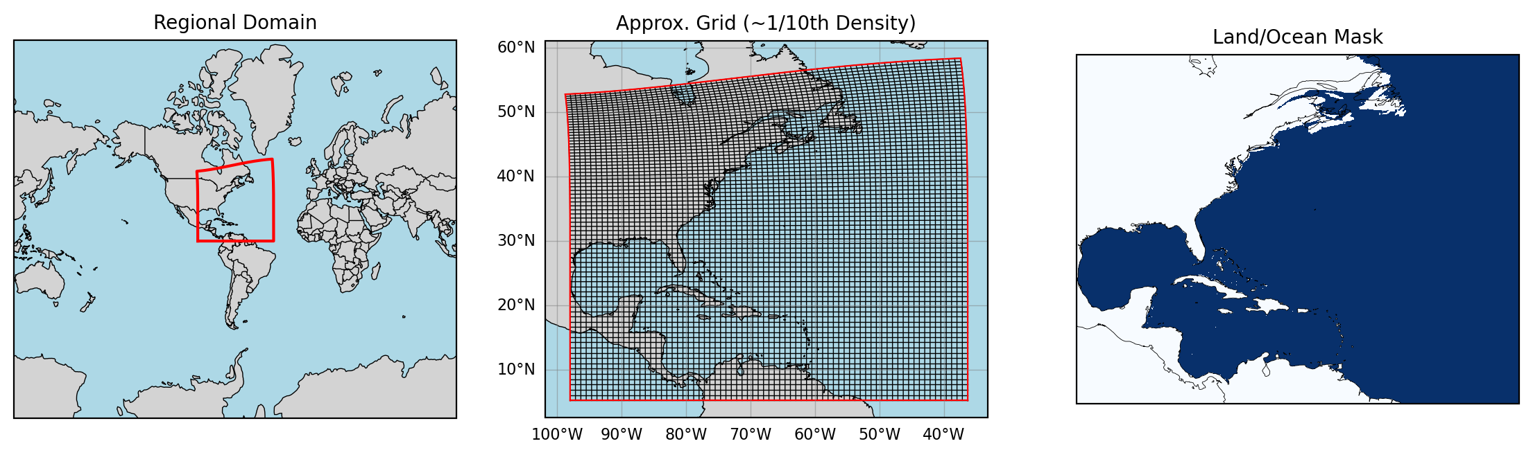
Plotting Regional MOM6 Output#
We will primarily look at the surface fields and some of the monthly full domain fields in this notebook.
Xarray comes with great default plotting wrappers that can do a lot! If you take an Xarray DataArray (one variable data structure) and call
xr.DataArray.plot()
it will usually do a pretty good job! Here we’ll walk through some powerful ways to use this plot wrapper, and we provide some additional functions to help the plotting along!
Simple plotting with Xarray#
By default, these files are all loaded in as Datasets which store a large set of variables with a variety of shared coordinates/dimensions.
When plotting, we need to reduce this space to a single variable. If we want to plot a spatial field we need one time step, and if we want to plot a timeseries, we need to average over the spatial dimensions (this is a bit more complicated than it might seem because the grid cells are not all the same size).
Let’s use some basic Xarray plotting to look at a surface field:
## Select a single variable at a single time
sst = sfc_data["tos"].isel(time=0)
sst.plot(cmap="viridis", vmin=-1.9, vmax=30)  # approx. color bar bounds for temp
# Note that it automatically labels with coordinate names and attributes.
<matplotlib.collections.QuadMesh at 0x7f4bf93f6fd0>
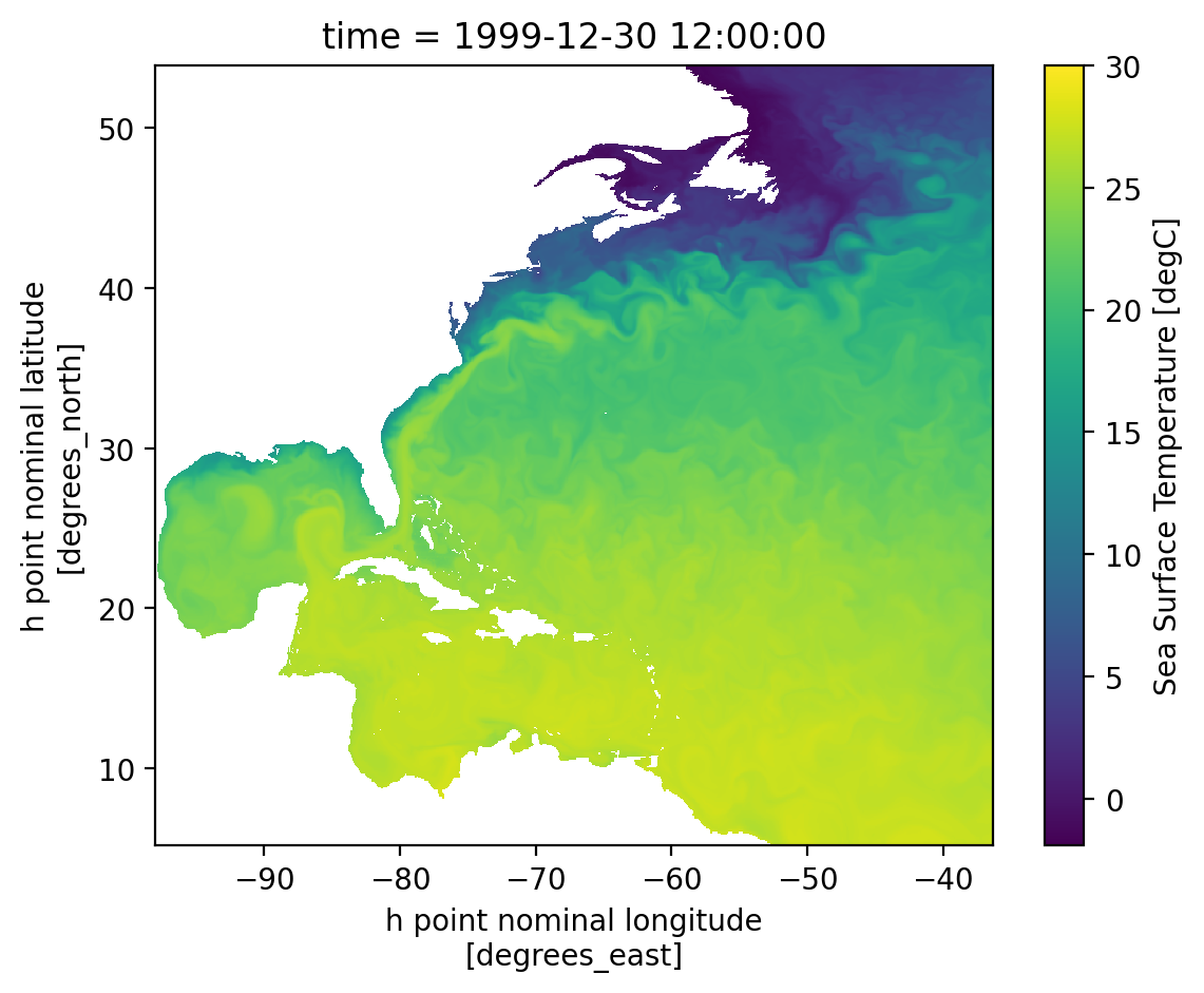
Looks good! But from above we know we want to plot with geolon and geolat for an accurate map. We can also choose some different color maps and projections. Let’s use some regional_utils to get this done.
## Select a single variable at a single time
sst = sfc_data["tos"].isel(time=0)

coords = utils.chooseGeoCoords(sst.dims)
lat = static_data[coords["latitude"]]
lon = static_data[coords["longitude"]]

sst = sst.assign_coords({"lon": lon, "lat": lat})

cmap = utils.chooseColorMap(sst.name)

cbar_levels = utils.chooseColorLevels(
    sst.min().compute().item(),
    sst.max().compute().item(),
)

# Create the plot with projection
fig = plt.figure(dpi=200)
ax = plt.axes(projection=ccrs.Mercator())

# Plot the data
p = sst.plot(
    x="lon",
    y="lat",
    cmap=cmap,
    levels=cbar_levels,
    transform=ccrs.PlateCarree(),
    ax=ax,
    add_colorbar=True,
)

# Add coastlines - now this should work
ax.coastlines(resolution="50m", color="black", linewidth=0.3)

plt.show()
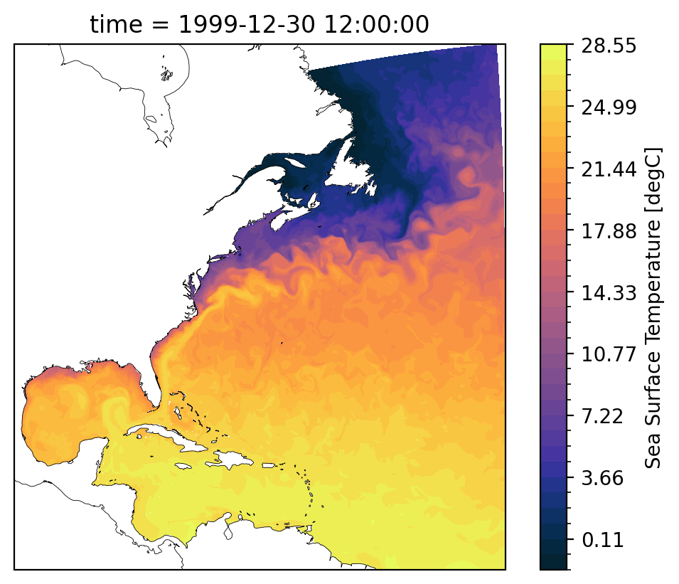
Looks good! Doing all this setup everytime would be cumbersome, so we wrapped it in a function utils.plotLatLonField.
Please go check it out and see what’s going on behind the scenes. It also can calculate statistics for the field taking into account area/volume weights.
MOM6 Output - Surface Fields#
The cells below visualize the mean state and the std of the fields over the full time given.
Show code cell source
Hide code cell source
## Ploting basic surface state variables
add_stats = True
time_bounds = (
    sfc_data["time"][0].compute().item(),
    sfc_data["time"][-1].compute().item(),
)

for var in sfc_variables:
    if var not in list(sfc_data.variables):
        print(f"Variable '{var}' not in given sfc_data. It will not be plotted.")
        sfc_variables.remove(var)


print(f"Taking mean and std dev from {time_bounds[0]} to {time_bounds[-1]}")
for var in sfc_variables:
    field = sfc_data[var]

    coords = utils.chooseGeoCoords(field.dims)
    areacello = utils.chooseAreacello(field.dims)

    mean = field.mean(dim="time", skipna=True).compute()
    std = field.std(dim="time", skipna=True).compute()
    mean.attrs = field.attrs
    std.attrs = field.attrs
    mean.attrs["long_name"] = f"Mean {field.long_name}"
    std.attrs["long_name"] = f"Std Dev {field.long_name}"

    utils.plotLatLonField(
        mean,
        latitude=static_data[coords["latitude"]],
        longitude=static_data[coords["longitude"]],
        stats=add_stats,
        area_weights=static_data[areacello],
        save=save_figs,
        save_path=image_output_dir,
    )
    plt.show()

    utils.plotLatLonField(
        std,
        latitude=static_data[coords["latitude"]],
        longitude=static_data[coords["longitude"]],
        stats=add_stats,
        area_weights=static_data[areacello],
        save=save_figs,
        save_path=image_output_dir,
    )
    plt.show()
Taking mean and std dev from 1999-12-30 12:00:00 to 2000-11-28 12:00:00
/glade/work/ajanney/conda-envs/cupid-analysis/lib/python3.11/site-packages/dask/array/numpy_compat.py:57: RuntimeWarning: invalid value encountered in divide
  x = np.divide(x1, x2, out)
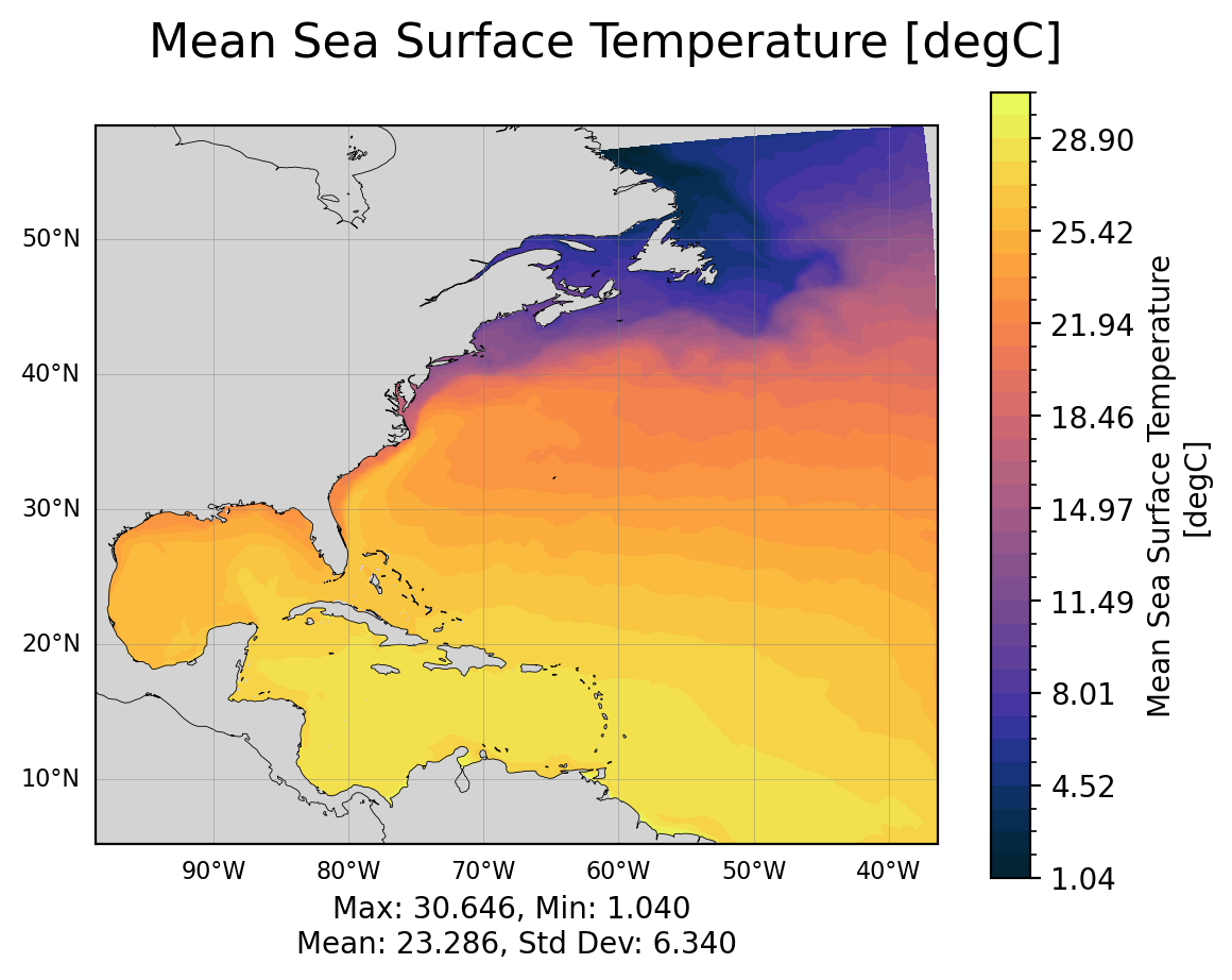
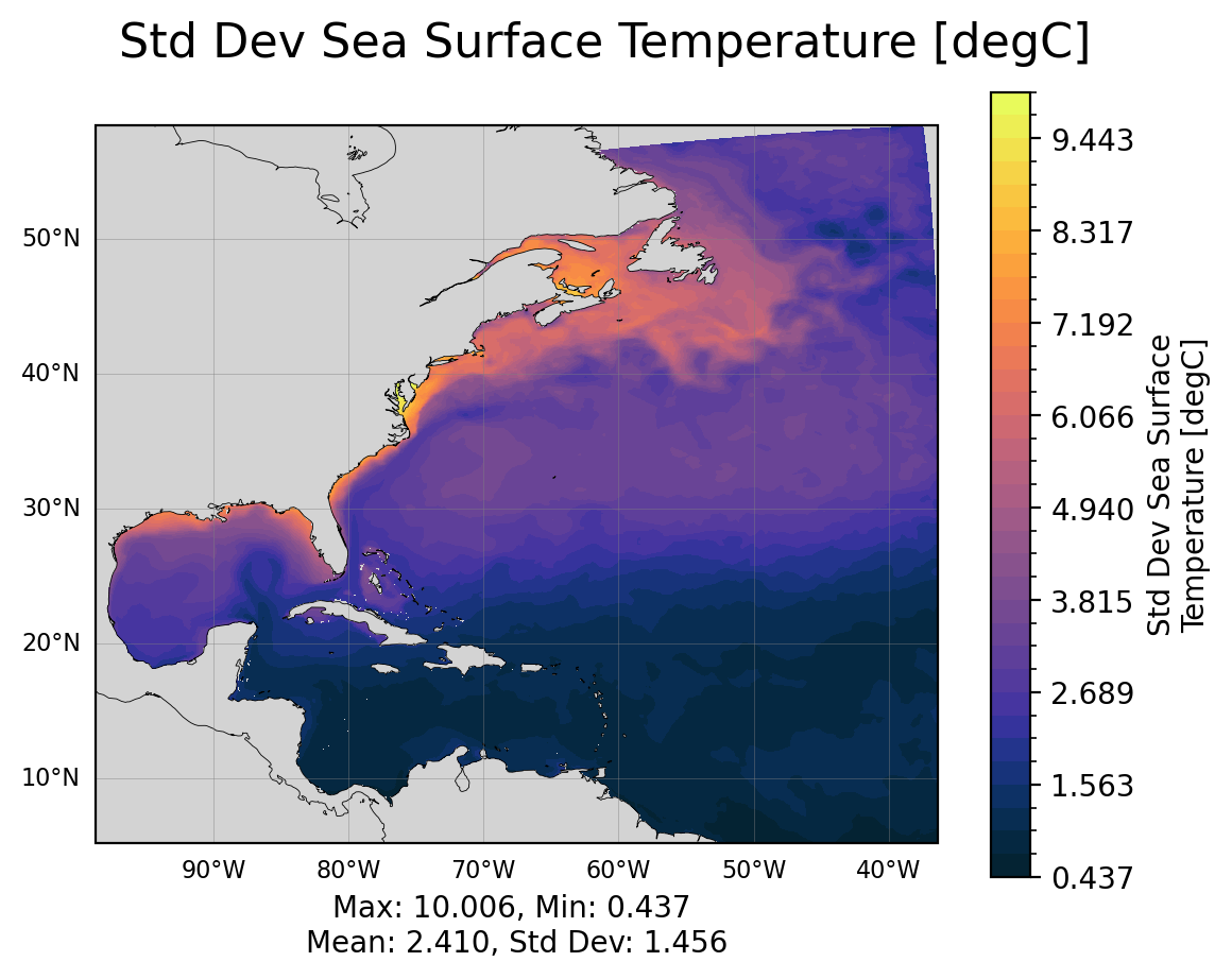
Area Weighted Averages and Timeseries#
Calculating and plotting timeseries can also be complicated. We need to be careful when taking an average of the fields that we take weighted statistics because the grid cells are not guaranteed to be constant area or volume.
The information we need for these weighted averages is contained in the areacello* variables (in static_data) and the volcello variable (in native_data and monthly_data).
We have to pay attention to coordinates and dimensions because of MOM6’s staggered grid (see how we choose the geolon/lat coords above).
Note: These timeseries may be less helpful for shorter runs, but see what they reveal!
Show code cell source
Hide code cell source
for var in sfc_variables:
    field = sfc_data[var]
    areacello_var = utils.chooseAreacello(field.dims)

    utils.plotAvgTimeseries(
        sfc_data[var],
        static_data[areacello_var],
        save=save_figs,
        save_path=image_output_dir,
    )
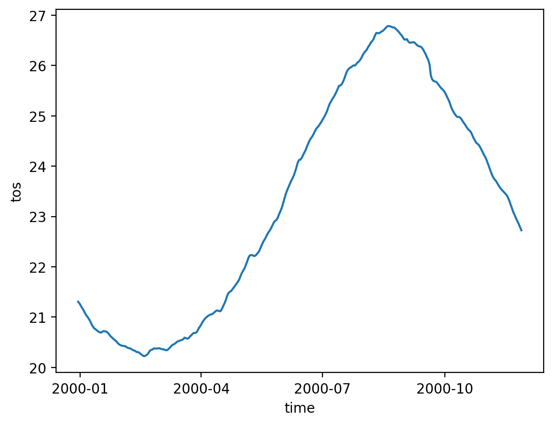
Viewing Full Domain Monthly Output#
Let’s look at the monthly output. When using longer runs (years or decades). These hold a lot more information about how your model is evolving and performing over time. For shorter runs (like many regional models often are), we may only have a handful of monthly output timesteps.
Xarray has some very useful methods for visualizing multiple levels and easily plotting them using the col and col_wrap keywords.
**Note: ** none of the following plots are saved. If you want to save them, rerun the first few cells of the notebook and manually save these.
for var in monthly_variables:
    if var not in list(monthly_data.variables):
        print(f"Variable '{var}' not in given monthly_data. It will not be plotted.")
        monthly_variables.remove(var)

## Let's only look at one variable for now (this plotting can be slow)
for var in monthly_variables[0:1]:
    # Look at only the first time step for now
    field = monthly_data[var].isel(time=0)

    cmap = utils.chooseColorMap(var)
    levels = utils.chooseColorLevels(
        field.min().compute().item(),
        field.max().compute().item(),
    )

    subplot_kwargs = {
        "projection": ccrs.Mercator(),
    }

    p = field.plot(
        col="z_l",
        col_wrap=5,
        cmap=cmap,
        levels=levels,
        transform=ccrs.PlateCarree(),
        subplot_kws=subplot_kwargs,
    )
    plt.suptitle(f"{var} at depths", y=1.0, fontsize=20)

    for ax in p.axs.flat:
        ax.coastlines(resolution="50m", color="black", linewidth=0.3)
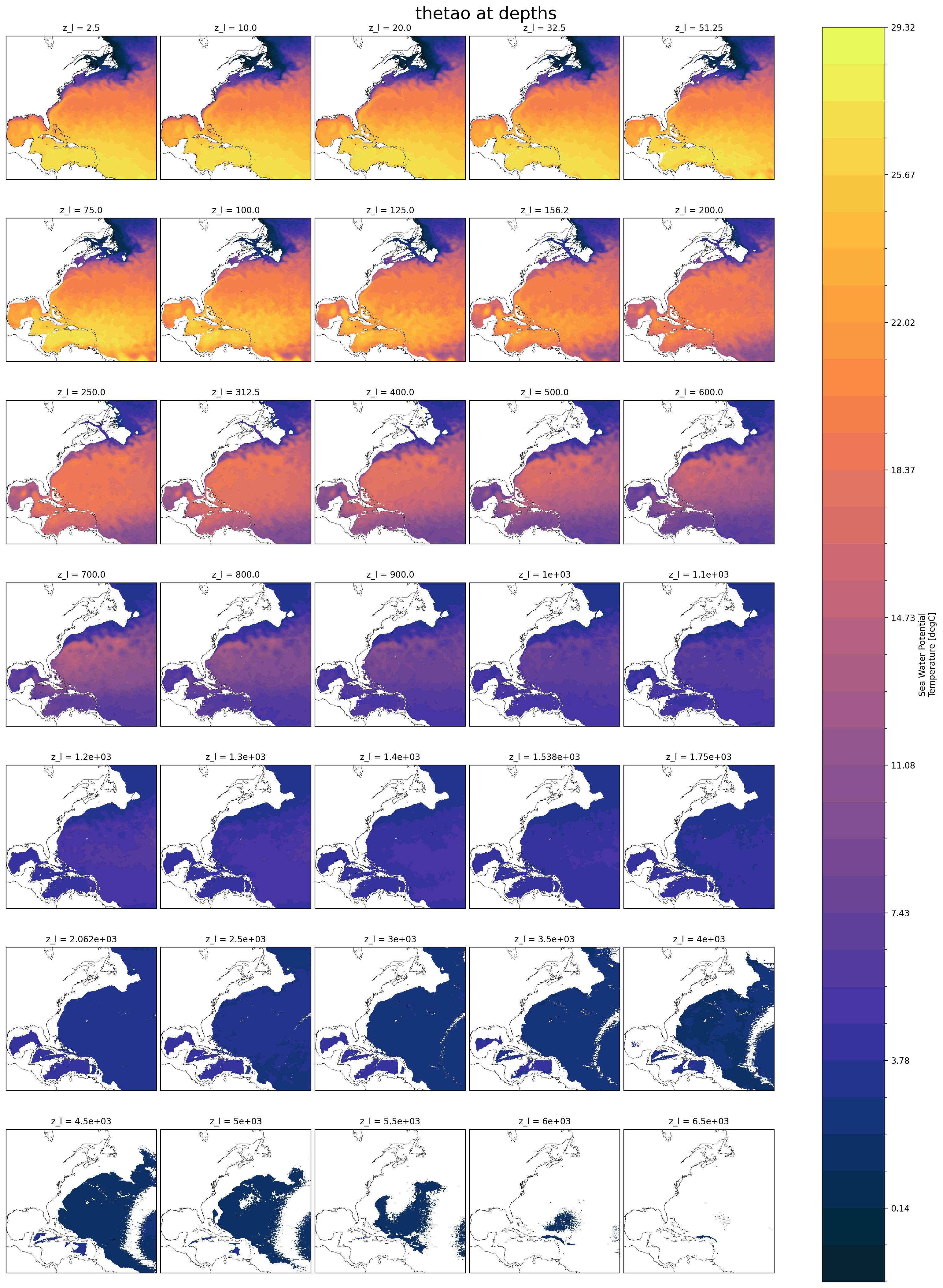
Vertical Profiles#
Another useful tool, sometimes we want to look at the vertical profile of something like salinity or temperature. Be careful to use area weighted averages here. (This could be a tool in regional_utils, but it’s not too much code, you decide!)
for var in monthly_variables[0:1]:  # only one variable again, make it more!
    # Look at only the first time step for now
    field = monthly_data[var].isel(time=0)

    area_weights = utils.chooseAreacello(field.dims)
    field_weighted = field.weighted(static_data[area_weights])

    mean_vars = [dim for dim in field.dims if dim != "z_l"]
    field_mean = field_weighted.mean(mean_vars)

    field_mean.plot(y="z_l", yincrease=False)
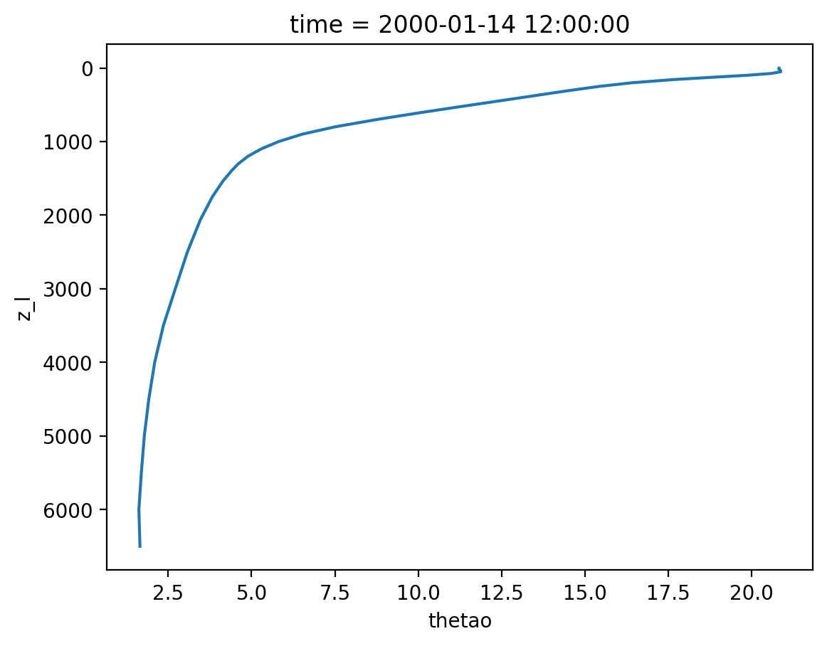
Bonus: Interpolating Levels and Slices#
We successfully plotted different levels above, we can also plot vertical slices. In both cases, we might run into an issue where we want to interpolate to a depth or lat/lon that is not explicitly resolved in the model. We can write our own tailored methods for this, but for simple visual inspection/comparison Xarray tools work well!
monthly_data["z_l"]
<xarray.DataArray 'z_l' (z_l: 35)> Size: 280B
array([2.5000e+00, 1.0000e+01, 2.0000e+01, 3.2500e+01, 5.1250e+01, 7.5000e+01,
       1.0000e+02, 1.2500e+02, 1.5625e+02, 2.0000e+02, 2.5000e+02, 3.1250e+02,
       4.0000e+02, 5.0000e+02, 6.0000e+02, 7.0000e+02, 8.0000e+02, 9.0000e+02,
       1.0000e+03, 1.1000e+03, 1.2000e+03, 1.3000e+03, 1.4000e+03, 1.5375e+03,
       1.7500e+03, 2.0625e+03, 2.5000e+03, 3.0000e+03, 3.5000e+03, 4.0000e+03,
       4.5000e+03, 5.0000e+03, 5.5000e+03, 6.0000e+03, 6.5000e+03])
Coordinates:
  * z_l      (z_l) float64 280B 2.5 10.0 20.0 32.5 ... 5.5e+03 6e+03 6.5e+03
Attributes:
    units:      meters
    long_name:  Depth at cell center
    axis:       Z
    positive:   down
edges: z_i- z_l: 35
- 2.5 10.0 20.0 32.5 51.25 75.0 ... 4.5e+03 5e+03 5.5e+03 6e+03 6.5e+03
array([2.5000e+00, 1.0000e+01, 2.0000e+01, 3.2500e+01, 5.1250e+01, 7.5000e+01, 1.0000e+02, 1.2500e+02, 1.5625e+02, 2.0000e+02, 2.5000e+02, 3.1250e+02, 4.0000e+02, 5.0000e+02, 6.0000e+02, 7.0000e+02, 8.0000e+02, 9.0000e+02, 1.0000e+03, 1.1000e+03, 1.2000e+03, 1.3000e+03, 1.4000e+03, 1.5375e+03, 1.7500e+03, 2.0625e+03, 2.5000e+03, 3.0000e+03, 3.5000e+03, 4.0000e+03, 4.5000e+03, 5.0000e+03, 5.5000e+03, 6.0000e+03, 6.5000e+03]) - z_l(z_l)float642.5 10.0 20.0 ... 6e+03 6.5e+03
- units :
- meters
- long_name :
- Depth at cell center
- axis :
- Z
- positive :
- down
- edges :
- z_i
array([2.5000e+00, 1.0000e+01, 2.0000e+01, 3.2500e+01, 5.1250e+01, 7.5000e+01,
       1.0000e+02, 1.2500e+02, 1.5625e+02, 2.0000e+02, 2.5000e+02, 3.1250e+02,
       4.0000e+02, 5.0000e+02, 6.0000e+02, 7.0000e+02, 8.0000e+02, 9.0000e+02,
       1.0000e+03, 1.1000e+03, 1.2000e+03, 1.3000e+03, 1.4000e+03, 1.5375e+03,
       1.7500e+03, 2.0625e+03, 2.5000e+03, 3.0000e+03, 3.5000e+03, 4.0000e+03,
       4.5000e+03, 5.0000e+03, 5.5000e+03, 6.0000e+03, 6.5000e+03])
- z_lPandasIndex
PandasIndex(Index([   2.5,   10.0,   20.0,   32.5,  51.25,   75.0,  100.0,  125.0, 156.25,
        200.0,  250.0,  312.5,  400.0,  500.0,  600.0,  700.0,  800.0,  900.0,
       1000.0, 1100.0, 1200.0, 1300.0, 1400.0, 1537.5, 1750.0, 2062.5, 2500.0,
       3000.0, 3500.0, 4000.0, 4500.0, 5000.0, 5500.0, 6000.0, 6500.0],
      dtype='float64', name='z_l'))
- units :
- meters
- long_name :
- Depth at cell center
- axis :
- Z
- positive :
- down
- edges :
- z_i
## Plot a specific depth
field = monthly_data["thetao"].isel(time=0)
field = field.interp(
    z_l=550, method="linear"
)  # you may choose a different depth if you want to test the interpolation

coords = utils.chooseGeoCoords(field.dims)
areacello = utils.chooseAreacello(field.dims)

utils.plotLatLonField(
    field,
    latitude=static_data[coords["latitude"]],
    longitude=static_data[coords["longitude"]],
    stats=True,
    area_weights=static_data[areacello],
    save=save_figs,
    save_path=image_output_dir,
)
plt.show()
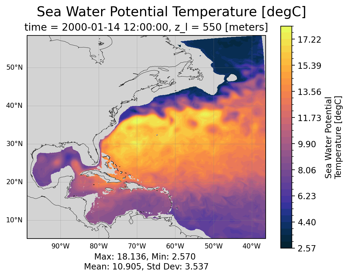
Let’s try it with a vertical slice now too!#
field = monthly_data["thetao"].isel(time=0)
x_var = "xh" if "xh" in field.dims else "xq"
longitude = np.mean(field[x_var].to_numpy())
vertical = field.interp({x_var: longitude})
levels = np.linspace(
    vertical.min().compute().item(), vertical.max().compute().item(), 35
)
vertical.plot(
    yincrease=False,
    levels=levels,
)
<matplotlib.collections.QuadMesh at 0x7f4c18c4d3d0>