Running a CUPiD Example

CUPiD provides examples of configuration files to allow users to look at a variety of diagnostics in CUPiD/examples. These examples are designed to be run on the NCAR supercomputers, using output curated from CESM development runs and stored in /glade/campaign/cesm/development/cross-wg/diagnostic_framework/CESM_output_for_testing/. The provided configuration files also act as templates for the CESM workflow, as discussed in the CUPiD project pages.

Note: we actually access the example output through the CROCODILE workshop directory for simplicity: /glade/campaign/cgd/oce/projects/CROCODILE/workshops/2025/Diagnostics/CESM_Output/. It just links back to CESM_output_for_testing.

There is a regional_ocean example in CUPiD that provides diagnostics for a 10-month CESM run created with CrocoDash. This run uses a 1/12° grid over the northwest Atlantic domain, and includes ocean biogeochemistry tracers from the Marine Biogeochemistry library (MARBL). (The compset used was 1850_DATM%JRA_SLND_SICE_MOM6%MARBL-BIO_SROF_SGLC_SWAV_SESP.)

For this exercise, we will run the regional_ocean example in CUPiD. This includes four notebooks:

• Regional_Ocean_Report_Card.ipynb: basic plotting and analysis utilities, primarily focused on surface fields.

• Regional_Ocean_Animations.ipynb: create animations.

• Regional_Ocean_Atmospheric_Forcing.ipynb: look at atmospheric forcing at the surface.

• Regional_Ocean_OBC.ipynb: visualize surface fields and open boundary conditions.

Task 2: Let’s Run CUPiD

Navigate to the examples subdirectory of your installation of CUPiD and look at what’s inside:

cd ${CUPID_ROOT}/examples
ls

Output

additional_metrics  external_diag_packages  key_metrics  regional_ocean

We will be using the regional_ocean example for this demo and the workshop:

cd regional_ocean

2.1 Confirm the Conda Environments Installed Correctly

For a standalone CUPiD run (as opposed to running it from a CESM case), run the cupid-diagnostics command from the same directory as a config.yml file. CUPiD will create a computed_notebooks directory for output. This command will only be recognized in the (cupid-infrastructure) environment, so let’s make sure the (cupid-infrastructure) and (cupid-analysis) conda environments are fully installed for everyone.

conda activate cupid-infrastructure
which cupid-diagnostics

If the environment installed correctly, which will return a path to cupid-diagnostics. If the environment did not install correctly, which will return an error like which: no cupid-diagnostics in [long list of directories].

Checkpoint #3

At this point the following should all be true:

1. your terminal is in CUPiD’s examples/regional_ocean directory,

2. the (cupid-infrastructure) conda environment is active, and

3. the which cupid-diagnostics command found the cupid-diagnostics script.

2.2 Time to Run CUPiD!

🚨 Conda and Jupyter might be Butting Heads 🚨

Before moving on, we want to make sure Jupyter can recognize the cupid-analysis environment that will run all of the notebooks. This may not be an issue for you, but just to be safe, follow the steps below.

conda activate cupid-analysis
python -m ipykernel install --user --name=cupid-analysis
conda deactivate  # or `conda activate cupid-infrastructure`

Now you should be back in the cupid-infrastructure environment and ready to rumble.

It’s finally time to run CUPiD! From the same ${CUPID_ROOT}/examples/regional_ocean directory, run on one processor with:

cupid-diagnostics --serial

This step might take some time, and we can track the progress with the output to terminal. If you notice an error about CUPiD not being able to find the (cupid-analysis) environment, make sure to check the red alert box above and install the ipykernel.

The notebooks will be run in nblibrary and then copied to computed_notebooks/ocn under the example directory. If you want to rerun the notebooks, make sure to manually copy the regional_utils.py file with:

cp ../../nblibrary/ocn/regional_utils.py computed_notebooks/ocn/

more on this and cupid-webpage below.

CUPiD Configuration

While we’re waiting for CUPiD, let’s revisit the famous config.yml file. It’s delineated

data_sources Section

The first section in the config.yml file is data_sources:

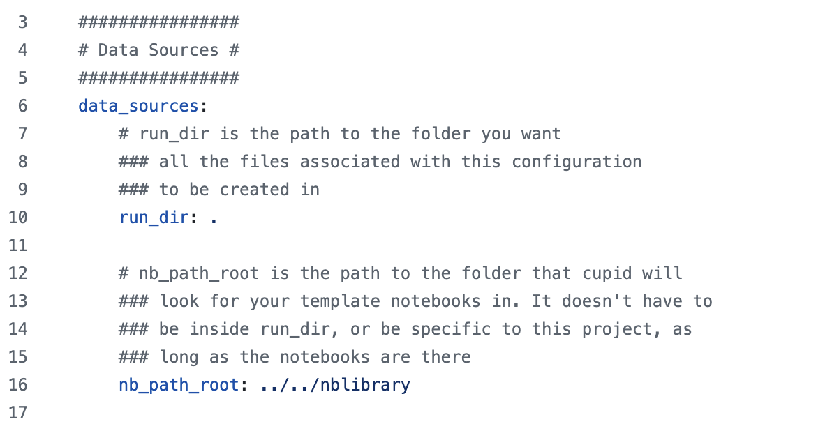
This typically does not need to be edited by the user, and may be removed in favor of command-line arguments to the cupid-diagnostics script. It points CUPiD to the notebook library and also tells CUPiD where to execute the notebooks (we want the notebooks to be run in the output directory rather than the nblibrary directory).

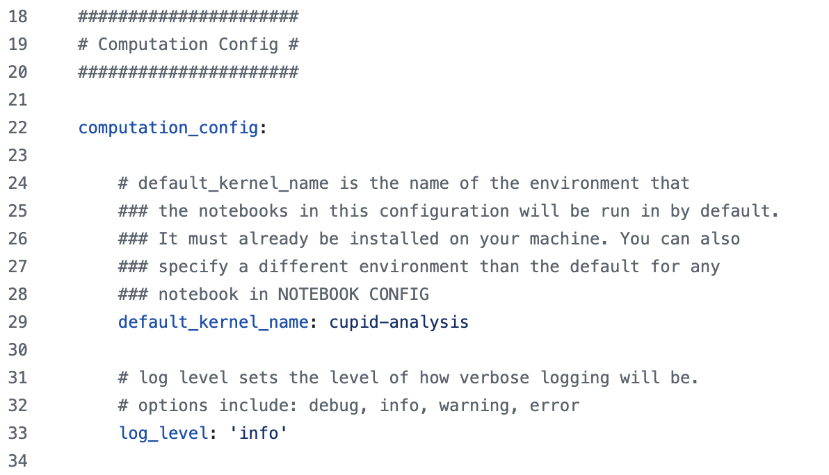
computation_config Section

Much like the data_sources section, this section typically does not need to be modified by users and may turn into command-line arguments. It provides the name of the conda environment to run notebooks in by default (users can specify different environments for individual notebooks), and it also sets logging information:

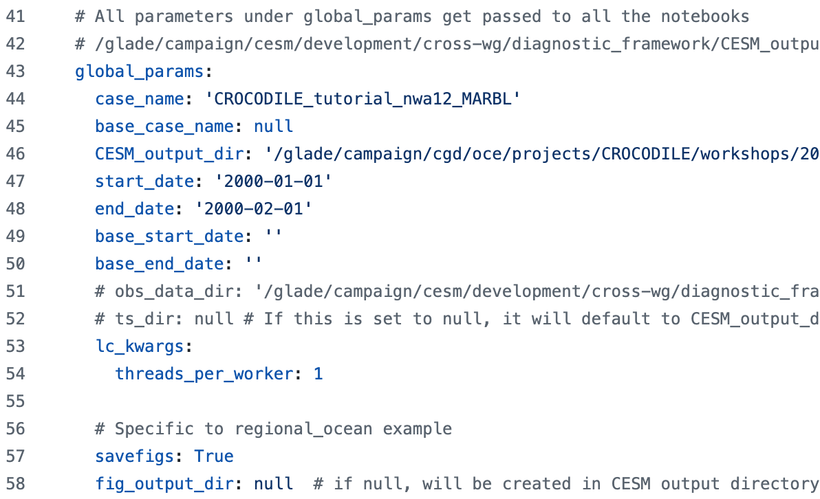
global_params Section

There are some parameters that are passed to every notebook. These are typically variables associated with the runs being compared (things like CESM case names, location of data, length of the run, and so on). For regional_ocean, there are some parameters we want to pass to every ocean notebook and they are included here as well:

time_series Section

One of the data standardization tasks CUPiD does is converting CESM history files to time series files (rather than have many variables at a single time level, these files are a single variable at many time levels). The notebooks provided for this tutorial read history files, and the interface for this section is still under development, so we won’t spend much time discussing it.

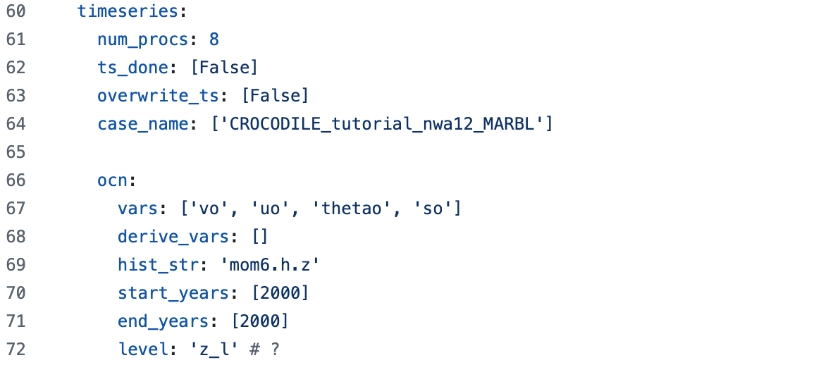
Want to generate a timeseries?

Note that the timeseries output directory ts_dir is not instantiated in this example. You are able to create timeseries files, but you are not able to save them to the CESM_output_dir as you normally would because we only have read permissions there.

If you want to run the timeseries tool, set ts_dir: /glade/derecho/scratch/${USER}/archive (or another directory you have write access to) and then run

cupid-timeseries

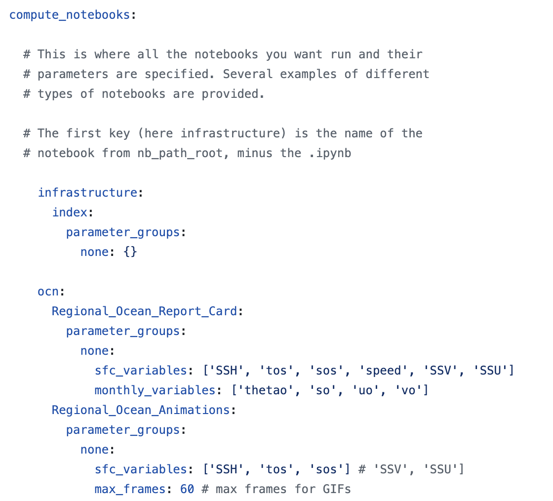
compute_notebooks Section

This section tells CUPiD what notebooks to run, and what parameters should be passed to that notebook in addition to the ones listed in global_params. CUPiD will always run the infrastructure section, and the user can specify what components (atm, ocn, lnd, etc) should also be run. By default, CUPiD will run all the notebooks in this section.

The first key under each component (e.g. Regional_Ocean_Report_Card) is the name of a notebook, and CUPiD will look in nblibrary/{component} for that file. In this example, CUPiD will run nblibrary/atm/Regional_Ocean_Report_Card.ipynb. You can provide more than one notebook per component.

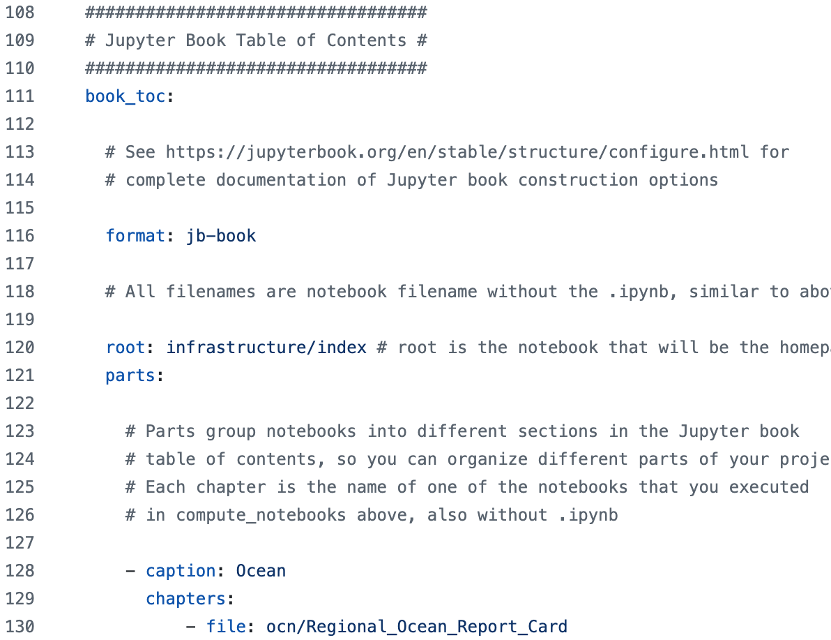
book_toc Section

After running all the notebooks specified in compute_notebooks, CUPiD can use Jupyter Book to create a website. Unfortunately there is not a great way to view HTML files that are stored on the NCAR super computers, so for this tutorial we will look at the notebooks that have been executed.

To build the website, however, the book_toc section lays out how to organize the notebooks into different chapters. Our examples organize the pages by component, but in other cases it may make sense to group notebooks differently (e.g. global surface plots in one section, time series plots of global means in another).

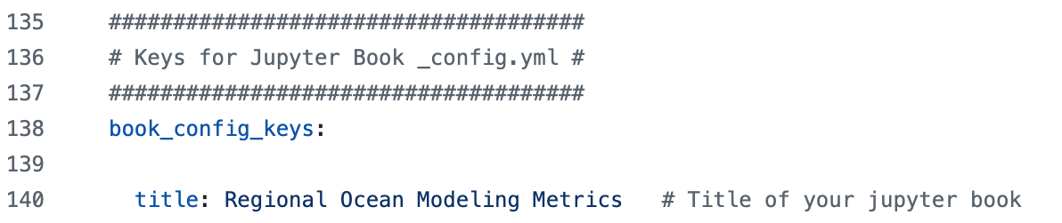
book_config_keys Section

This section is used to set the title of the Jupyter Book webpage. It should probable be combined with the book_toc section, or maybe it should be a command line argument instead.

Where are my notebooks?

Remember that the notebooks all run in nblibrary, but after cupid-diagnostics has finished, the notebooks are all copied over the the run_dir in the config file (in this case the same directory as the config). This primarily matters for re-running notebooks when we would need to copy over any dependencies (e.g. nblibrary/regional_ocean.utils.py) and be aware of relative paths.

Brief overview of the notebooks

To the JupyterHub! Navigate to nblibrary to follow along and we’ll take a look at what our output should look like.

We can also take a sneak peak at the CrocoGallery CUPiD_output page before your output is done generating.

Final Task: Now it’s your turn!

The power of CUPiD now lies in your hands (don’t spend it all in one place, or do, it’s reusable)!

Please mess with this config file, change variables, adjust paths! Feel free to go in an modify any code you like.

If you want to run the CUPiD notebooks on your CESM output from the tutorials earlier in the week, it can be done in a few simple steps. In the same examples/regional_ocean directory:

1. mv computed_notebooks computed_notebooks.example - try not to override diagnostic output, your future self will thank you!

2. Modify config.yml paths/variables:

   1. Global Params:case_name and CESM_output_dir

   2. Notebook Params: mom6_input_dir - look for ocnice from CrocoDash!

3. Run cupid-diagnostics --serial - some of the output may look a little different becaue we’re working with days/weeks not months.

4. Let us know if you run into any issues!

Want to generate a CUPiD webpage of your output?

We recommend viewing the completed notebooks in JupyterHub. This is the easiest way to see CUPiD output on the NCAR super computer, and also makes it easy to re-run the notebooks manually if you want to play with the output.

Note: make sure to select the cupid-analysis kernel in the top right if you want to rerun the notebooks.

If you want to use CUPiD’s webpage feature, however, run

cupid-webpage

after cupid-diagnostics completes. Like cupid-diagnostics, this command is part of the (cupid-infrastructure) environment and should be run from the directory containing config.yml.

Unfortunately, it is not easy to view webpages on the NCAR super computer. Your best bet is probably copying the entire computed_notebooks/_build/html directory to your local computer. More options are discussed in the CUPiD documentation for Looking at Output.

You can transfer the files to your personal computer using a tool like scp or rsync:

scp USERNAME@casper.hpc.ucar.edu:/glade/work/USERNAME/crocodile_2025/CUPiD/examples/computed_notebooks/_build /path/on/personal/computer

Alternatively, make sure to attend Sam Rabin’s lecture on VSCode tools for another fancy way of viewing HTML files!