Bering Sea: ocean, sea ice and waves — workshop diagnostics

A guided look at a coupled MOM6 + CICE + WW3 regional run of the Bering Sea, aimed at someone who knows ocean models but not sea ice or waves.

Everything is daily-mean output from the case you built! CICE daily fields carry a _d suffix (aice_d, hi_d, ...) because they come from CICE history stream 2.

The physical story this run is built to show¶

Waves radiate into the ice edge and fracture large floes into smaller ones. Smaller floes have more edge per unit area, and ice melts laterally from its edges — so a broken-up ice cover melts faster than a solid one. Faster melt opens more water, longer open-water fetch builds bigger waves, which break more ice. That feedback is the marginal ice zone (MIZ), and representing it is the entire reason a model carries a floe size distribution (FSD) instead of just ice concentration.

Two caveats, stated up front¶

No WW3 boundary spectra. This configuration has no wave forcing at the open boundaries, so waves are generated only by winds inside the domain. Real swell travels hundreds of km into pack ice and is absent here. Wave heights, and therefore fracturing, are underestimates.
327 cells carry a garbage wave height (~2.5e15 m). It is the same 327 cells every day — a static artifact where the WW3 and CICE masks disagree, not evolving physics. The other 8733 wet cells are a sensible 0-9 m. WAVE_MAX below masks them; do not remove that mask without checking.

import os
from pathlib import Path

import cartopy.crs as ccrs
import matplotlib.pyplot as plt
import numpy as np
import xarray as xr
from matplotlib import animation
from IPython.display import HTML

CASE    = "bering_ocn_wav_ice.001"
# CESM's default short-term archive on Derecho (DOUT_S_ROOT). $SCRATCH points at your Derecho
# scratch from both Derecho and Casper. If you changed DOUT_S_ROOT, point ARCHIVE there instead.
ARCHIVE = Path(os.environ["SCRATCH"]) / "archive" / CASE

ICE_EDGE  = 0.15     # conventional ice-edge concentration
WAVE_MAX  = 100.0    # m -- above this is the mask artifact described above

ice = xr.open_mfdataset(sorted((ARCHIVE/"ice"/"hist").glob(f"{CASE}.cice.h1.*.nc")),
                        combine="by_coords", decode_times=True)
ocn = xr.open_mfdataset(sorted((ARCHIVE/"ocn"/"hist").glob(f"{CASE}.mom6.h.sfc.*.nc")),
                        combine="by_coords", decode_times=True)

LON, LAT = ice["TLON"].values, ice["TLAT"].values          # 2-D, (nj, ni)
NDAYS    = ice.sizes["time"]

# The case runs on a NO_LEAP calendar, so xarray decodes time to cftime objects, which matplotlib
# will not plot directly. Plot against a day index and label the ticks with date strings.
DAYS  = np.arange(NDAYS)
DATES = [str(t)[:10] for t in ice.time.values]

def datelabels(ax, every=None):
    every = every or max(1, NDAYS // 8)
    ax.set_xticks(DAYS[::every])
    ax.set_xticklabels(DATES[::every], rotation=45, ha="right", fontsize=8)
print(f"{NDAYS} daily frames | ice {dict(ice.sizes)}")
print("ocean sfc vars:", [v for v in ("tos","sos","mlotst","SSU","SSV") if v in ocn])

/glade/derecho/scratch/dbailey/tmp/ipykernel_4969/3540535680.py:16: FutureWarning: In a future version of xarray the default value for data_vars will change from data_vars='all' to data_vars=None. This is likely to lead to different results when multiple datasets have matching variables with overlapping values. To opt in to new defaults and get rid of these warnings now use `set_options(use_new_combine_kwarg_defaults=True) or set data_vars explicitly.
  ice = xr.open_mfdataset(sorted((ARCHIVE/"ice"/"hist").glob(f"{CASE}.cice.h1.*.nc")),
/glade/derecho/scratch/dbailey/tmp/ipykernel_4969/3540535680.py:18: FutureWarning: In a future version, xarray will not decode the variable 'average_DT' into a timedelta64 dtype based on the presence of a timedelta-like 'units' attribute by default. Instead it will rely on the presence of a timedelta64 'dtype' attribute, which is now xarray's default way of encoding timedelta64 values.
To continue decoding into a timedelta64 dtype, either set `decode_timedelta=True` when opening this dataset, or add the attribute `dtype='timedelta64[ns]'` to this variable on disk.
To opt-in to future behavior, set `decode_timedelta=False`.
  ocn = xr.open_mfdataset(sorted((ARCHIVE/"ocn"/"hist").glob(f"{CASE}.mom6.h.sfc.*.nc")),

31 daily frames | ice {'time': 31, 'nbnd': 2, 'nkice': 8, 'nksnow': 3, 'nkbio': 5, 'nkaer': 7, 'nj': 96, 'ni': 216, 'nvertices': 4, 'nc': 5, 'nf': 12}
ocean sfc vars: ['tos', 'sos', 'mlotst', 'SSU', 'SSV']

1. The setting: SST and where the ice is¶

Ocean and ice are on the same horizontal grid here, so they can be drawn together directly. The black contour is the ice edge, conventionally the 15% concentration line.

Note the ice sits where SST is at the freezing point (about -1.8 C for seawater) — ice and SST are not independent fields, they are two views of the same surface heat budget.

PROJ = ccrs.Stereographic(central_latitude=65.0, central_longitude=187.5)
XT   = ccrs.PlateCarree()      # data is in plain lon/lat (0-360)

def basemap(ax, title=""):
    ax.set_extent([LON.min(), LON.max(), LAT.min(), LAT.max()], XT)
    ax.coastlines("10m", linewidth=0.6)
    ax.set_facecolor("0.85")
    gl = ax.gridlines(draw_labels=True, linewidth=0.3, alpha=0.4)
    gl.top_labels = gl.right_labels = False
    ax.set_title(title, fontsize=11)

day = -1                                        # last day
sst  = ocn["tos"].isel(time=day).values
aice = ice["aice_d"].isel(time=day).values

fig, ax = plt.subplots(figsize=(11, 4.2), subplot_kw={"projection": PROJ},
                       constrained_layout=True)
basemap(ax, f"SST and ice edge — {str(ice.time.values[day])[:10]}")
pc = ax.pcolormesh(LON, LAT, sst, cmap="viridis", shading="nearest", transform=XT)
ax.contour(LON, LAT, aice, levels=[ICE_EDGE], colors="k", linewidths=1.6, transform=XT)
fig.colorbar(pc, ax=ax, label="SST (degC)", shrink=0.85)
plt.show()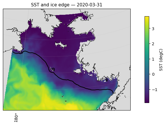

2. The movie: SST with ice concentration on top¶

Ice concentration is drawn as a translucent white overlay, so you see the ocean underneath and the ice pack riding on it. Watch the ice edge advance and flex with the weather.

With only a month of output this is short. The same cell will produce a full seasonal animation once the 12-month case finishes — nothing here depends on the run length.

fig, ax = plt.subplots(figsize=(6, 4.2), subplot_kw={"projection": PROJ},
                       constrained_layout=True)
basemap(ax)

vmin, vmax = np.nanpercentile(ocn["tos"].values, [1, 99])
sst_norm = plt.Normalize(vmin, vmax)
sst_cmap = plt.get_cmap("viridis")
ice_cmap = plt.get_cmap("Blues_r")
ICE_ALPHA = 0.75

# Two separate alpha-blended pcolormesh layers leave hairline white seams at every
# cell edge (an Agg antialiasing artifact when adjacent quads are only partially
# opaque) -- not fixed by antialiased=False, edgecolors, or gouraud shading. The
# fix is to pre-composite SST and ice into a single fully-opaque RGBA image and
# draw that as one mesh, so there is no partial-alpha quad-on-quad blending left
# for the renderer to seam.
def composite(t):
    sst = ocn["tos"].isel(time=t).values
    a   = ice["aice_d"].isel(time=t).values
    sst_rgb = sst_cmap(sst_norm(sst))[..., :3]
    ice_rgb = ice_cmap(plt.Normalize(0, 1)(np.clip(a, 0, 1)))[..., :3]
    ice_a   = np.where(a >= 0.05, ICE_ALPHA, 0.0)
    rgb   = ice_rgb * ice_a[..., None] + sst_rgb * (1 - ice_a[..., None])
    alpha = np.where(np.isnan(sst), 0.0, 1.0)       # land/missing -> transparent
    return np.dstack([rgb, alpha])

pc = ax.pcolormesh(LON, LAT, composite(0), shading="nearest", transform=XT)
sm = plt.cm.ScalarMappable(norm=sst_norm, cmap=sst_cmap)     # for the colorbar only
fig.colorbar(sm, ax=ax, label="SST (degC)", shrink=0.85)

def frame(t):
    pc.set_array(composite(t))
    ax.set_title(f"SST + sea ice concentration — {str(ice.time.values[t])[:10]}", fontsize=11)
    return (pc,)

anim = animation.FuncAnimation(fig, frame, frames=NDAYS, interval=400, blit=False)
plt.close(fig)
HTML(anim.to_jshtml())

OUT = Path.cwd() / "bering_sst_ice_animation.mp4"
anim.save(OUT, writer=animation.FFMpegWriter(fps=1000/400, bitrate=1800))
print(f"saved {OUT}")

saved /glade/work/dbailey/bering/bering_sst_ice_animation.mp4

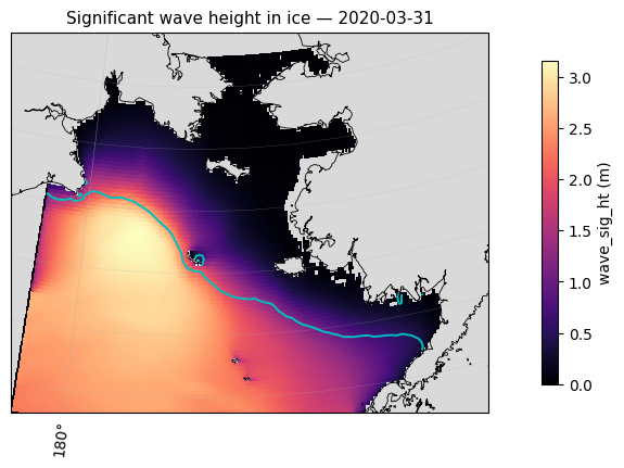
3. The wave field inside the ice¶

wave_sig_ht_d is significant wave height where there is ice — the quantity that drives fracturing.

Two things to look for. Wave height should decay going into the pack: ice damps waves, so the biggest values sit at the ice edge and fall off inward. And wave height should be episodic — calm for days, then a storm.

(The mask below removes the 327 artifact cells. n_bad is printed so you can confirm it is still the same small, constant number.)

wave = ice["wave_sig_ht_d"].where(ice["wave_sig_ht_d"] < WAVE_MAX)
n_bad = int((ice["wave_sig_ht_d"] >= WAVE_MAX).isel(time=0).sum())
print(f"masked artifact cells: {n_bad} (expected ~327, constant in time)")

fig, ax = plt.subplots(figsize=(11, 4.2), subplot_kw={"projection": PROJ},
                       constrained_layout=True)
basemap(ax, f"Significant wave height in ice — {str(ice.time.values[day])[:10]}")
pc = ax.pcolormesh(LON, LAT, wave.isel(time=day).values, cmap="magma",
                   shading="nearest", transform=XT)
ax.contour(LON, LAT, ice["aice_d"].isel(time=day).values, levels=[ICE_EDGE],
           colors="c", linewidths=1.4, transform=XT)
fig.colorbar(pc, ax=ax, label="wave_sig_ht (m)", shrink=0.85)
plt.show()

masked artifact cells: 0 (expected ~327, constant in time)

4. What the floe size distribution actually is¶

Ice concentration says how much ice. The FSD says how it is broken up.

afsd_d has an extra dimension nf — 12 floe-size categories, smallest to largest. For each grid cell it gives the fraction of ice area in each size class, so it is a histogram per cell. fsdrad_d collapses that to a single representative floe radius, which is the easy thing to map.

Below: a map of representative radius, then the full distribution at two contrasting points — one near the ice edge, one deep in the pack. Expect the edge to be shifted toward small floes.

fig, axs = plt.subplots(1, 2, figsize=(13, 4.0),
                        gridspec_kw={"width_ratios": [1.5, 1]}, constrained_layout=True)
axs[0].remove(); ax0 = fig.add_subplot(1, 2, 1, projection=PROJ)
basemap(ax0, f"Representative floe radius — {str(ice.time.values[day])[:10]}")

fsdrad = ice["fsdrad_d"].isel(time=day).where(ice["aice_d"].isel(time=day) > ICE_EDGE)
pc = ax0.pcolormesh(LON, LAT, fsdrad.values, cmap="cividis", shading="nearest", transform=XT)
fig.colorbar(pc, ax=ax0, label="fsdrad (m)", shrink=0.85)

# pick an edge cell and an interior cell from the same day
a = ice["aice_d"].isel(time=day).values
edge_mask = (a > ICE_EDGE) & (a < 0.5)
deep_mask = a > 0.95
jj, ii = np.where(edge_mask); je, ie = (jj[len(jj)//2], ii[len(ii)//2]) if len(jj) else (0, 0)
jj, ii = np.where(deep_mask); jd, idp = (jj[len(jj)//2], ii[len(ii)//2]) if len(jj) else (0, 0)

for (j, i), lab in [((je, ie), f"ice edge (aice={a[je, ie]:.2f})"),
                    ((jd, idp), f"interior (aice={a[jd, idp]:.2f})")]:
    axs[1].plot(np.arange(ice.sizes["nf"]), ice["afsd_d"].isel(time=day, nj=j, ni=i).values,
                marker="o", ms=4, label=lab)
    ax0.plot(LON[j, i], LAT[j, i], "o", mfc="none", mec="r", ms=9, mew=1.6, transform=XT)

axs[1].set_xlabel("floe size category (small -> large)")
axs[1].set_ylabel("areal fraction")
axs[1].set_title("floe size distribution", fontsize=11)
axs[1].legend(fontsize=8); axs[1].grid(alpha=0.3)
plt.show()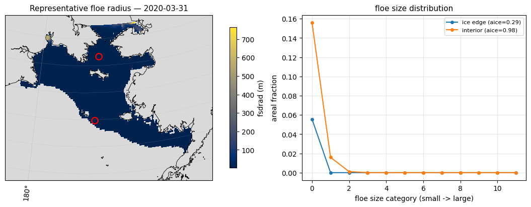

5. Which process is reshaping the floes?¶

This is the most diagnostic view. CICE reports the FSD tendency split by process, and they form a budget:

term	process
`dafsd_wave_d`	wave fracturing — the wave-to-ice coupling
`dafsd_weld_d`	welding: floes freezing back together in calm conditions
`dafsd_newi_d`	new ice formation
`dafsd_latg_d`	lateral growth
`dafsd_latm_d`	lateral melt

Wave fracturing has a characteristic signature: negative at large floe sizes, positive at small ones — area being moved down the size spectrum as big floes shatter. That sign pattern, not the magnitude, is the thing to recognise, and it is clearly visible in the left panel below.

The right panel puts fracturing activity next to peak wave height. Over only seven winter days these do not track each other cleanly — do not read a correlation into it. Fracturing depends on the wave spectrum reaching floes of a breakable size, not on peak height alone, and a week is far too short a sample. This panel becomes meaningful over the 12-month run.

Only dafsd_wave is on the daily stream here; the others default to monthly. Add them to user_nl_cice as 'mdxxx' if you want the full budget daily.

dw = ice["dafsd_wave_d"]
# domain-summed tendency per floe-size category, per day
prof = dw.sum(dim=("nj", "ni")).compute()

fig, axs = plt.subplots(1, 2, figsize=(12, 3.8), constrained_layout=True)

for t in range(NDAYS):
    axs[0].plot(np.arange(ice.sizes["nf"]), prof.isel(time=t).values,
                marker="o", ms=3, alpha=0.8, label=str(ice.time.values[t])[:10])
axs[0].axhline(0, color="k", lw=0.8)
axs[0].set_xlabel("floe size category (small -> large)")
axs[0].set_ylabel("domain-summed dafsd_wave (1/s)")
axs[0].set_title("wave fracturing moves area down the size spectrum", fontsize=11)
axs[0].legend(fontsize=7, ncol=2); axs[0].grid(alpha=0.3)

# how active is fracturing, day by day, vs how big the waves are
frac = np.abs(dw).sum(dim=("nf", "nj", "ni")).compute()
wmax = wave.max(dim=("nj", "ni")).compute()
ax2 = axs[1]
ax2.plot(DAYS, frac.values, "o-", color="tab:red", label="|dafsd_wave| (domain sum)")
ax2.set_ylabel("fracturing activity", color="tab:red")
ax2.tick_params(axis="y", labelcolor="tab:red")
ax3 = ax2.twinx()
ax3.plot(DAYS, wmax.values, "s--", color="tab:blue", label="max wave_sig_ht")
ax3.set_ylabel("max wave height (m)", color="tab:blue")
ax3.tick_params(axis="y", labelcolor="tab:blue")
ax2.set_title("fracturing activity vs wave height", fontsize=11)
ax2.grid(alpha=0.3)
datelabels(ax2)
plt.show()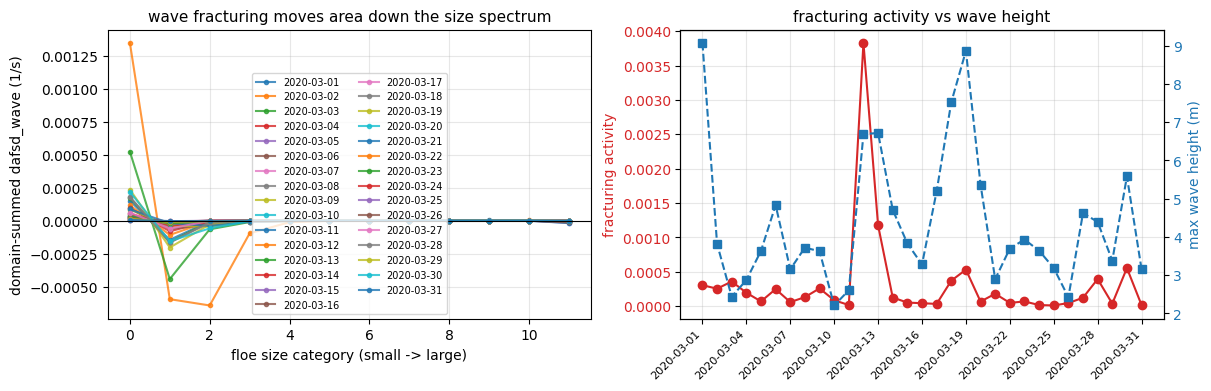

6. Domain-integrated time series¶

The summary numbers an oceanographer will want: how much ice there is, how thick, how broken up, and how energetic the waves are. Over a week these barely move; over a year they show the full advance and retreat.

ice area is concentration times cell area summed — the physically meaningful quantity, as opposed to extent (area of cells exceeding 15%), which is what satellite products usually report.

tarea = ice["tarea"].isel(time=0) if "time" in ice["tarea"].dims else ice["tarea"]

area = (ice["aice_d"] * tarea).sum(dim=("nj", "ni")).compute() / 1e12      # 10^6 km^2
vol  = (ice["hi_d"] * ice["aice_d"] * tarea).sum(dim=("nj", "ni")).compute() / 1e12  # 10^3 km^3
rad  = ice["fsdrad_d"].where(ice["aice_d"] > ICE_EDGE).mean(dim=("nj", "ni")).compute()
sst  = ocn["tos"].mean(dim=("yh", "xh")).compute()

fig, axs = plt.subplots(2, 2, figsize=(11, 6), constrained_layout=True, sharex=True)
for ax, y, lab in [(axs[0, 0], area, "ice area (10$^6$ km$^2$)"),
                   (axs[0, 1], vol,  "ice volume (10$^3$ km$^3$)"),
                   (axs[1, 0], rad,  "mean floe radius in pack (m)"),
                   (axs[1, 1], sst,  "domain-mean SST (degC)")]:
    ax.plot(DAYS[:y.sizes["time"]], y.values, "o-", ms=4)
    ax.set_ylabel(lab); ax.grid(alpha=0.3)
for ax in axs[1, :]:
    datelabels(ax)
plt.show()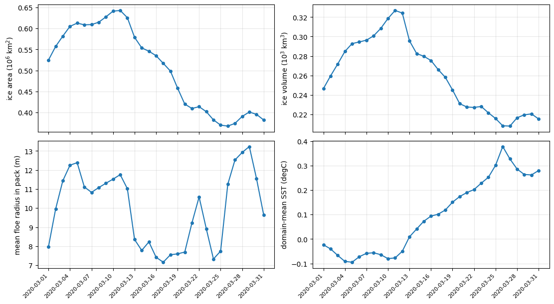

What to take away¶

Ice and SST are one system. Ice forms where the ocean is at freezing; the ice edge and the -1.8 C isotherm track each other.
The FSD is the ice cover’s grain size. Two cells with identical concentration can melt at very different rates depending on how broken up they are, because melt happens at floe edges.
dafsd_wave is the coupling term to watch. It is the only place in this model where the wave field changes the ice, and its negative-at-large / positive-at-small signature is the fingerprint of fracturing.
Remember what is missing. No wave forcing at the boundaries means no remotely generated swell, which is the dominant ice-breaking agent in the real Bering Sea. Treat the wave-ice coupling here as a demonstration of mechanism, not a quantitative result.

Next¶

A 12-month version of this case is being set up, which will make the animation in section 2 show a full ice advance and retreat, and turn section 6 into a real seasonal cycle.