Regional Ocean: Atmospheric Forcing¶

case_name = ""  # "/glade/campaign/cgd/oce/projects/CROCODILE/workshops/2025/Diagnostics/CESM_Output/"
CESM_output_dir = ""  # "CROCODILE_tutorial_nwa12_MARBL"

# As regional domains vary so much in purpose, simulation length, and extent, we don't want to assume a minimum duration
## Thus, we ignore start and end dates and simply reduce/output over the whole time frame for all of the examples given.
start_date = None  # "0001-01-01"
end_date = None  # "0101-01-01

save_figs = False
fig_output_dir = None

lc_kwargs = {}
serial = False

atm_variables = []  # ['tauuo', 'tauvo', 'hfds']
ocn_variables = []  # ['uo', 'vo', 'thetao']

# Parameters
case_name = "CROCODILE_tutorial_nwa12_MARBL"
CESM_output_dir = (
    "/glade/campaign/cgd/oce/projects/CROCODILE/workshops/2025/Diagnostics/CESM_Output/"
)
start_date = ""
end_date = ""
save_figs = True
fig_output_dir = None
lc_kwargs = {"threads_per_worker": 1}
serial = True
atm_variables = ["tauuo", "tauvo", "hfds"]
ocn_variables = ["uo", "vo", "thetao"]
subset_kwargs = {}
product = "/glade/work/ajanney/crocodile_2025/CUPiD/examples/regional_ocean/computed_notebooks//ocn/Regional_Ocean_Atmospheric_Forcing.ipynb"

Output directory is: /glade/campaign/cgd/oce/projects/CROCODILE/workshops/2025/Diagnostics/CESM_Output//CROCODILE_tutorial_nwa12_MARBL/ocn/hist/

case_output_dir = os.path.join(CESM_output_dir, case_name, "ocn", "hist")

# Xarray time decoding things
time_coder = xr.coders.CFDatetimeCoder(use_cftime=True)

## Static data includes hgrid, vgrid, bathymetry, land/sea mask
static_data = xr.open_mfdataset(
    os.path.join(case_output_dir, f"*static.nc"),
    decode_timedelta=True,
    decode_times=time_coder,
    engine="netcdf4",
)

# ## Surface Data
# sfc_data = xr.open_mfdataset(
#     os.path.join(case_output_dir, f"*sfc*.nc"),
#     decode_timedelta=True,
#     decode_times=time_coder,
#     engine="netcdf4",
# )

## Native Monthly Domain Data (and atm forcing)
monthly_data = xr.open_mfdataset(
    os.path.join(case_output_dir, f"*h.z*.nc"),
    decode_timedelta=True,
    decode_times=time_coder,
    engine="netcdf4",
)

## Native Monthly Domain Data (and atm forcing)
native_data = xr.open_mfdataset(
    os.path.join(case_output_dir, f"*native*.nc"),
    decode_timedelta=True,
    decode_times=time_coder,
    engine="netcdf4",
)

## Image/Gif Output Directory
if fig_output_dir is None:
    image_output_dir = os.path.join(
        "/glade/derecho/scratch/",
        os.environ["USER"],
        "archive",
        case_name,
        "ocn",
        "cupid_images",
    )
else:
    image_output_dir = os.path.join(fig_output_dir, case_name, "ocn", "cupid_images")
if not os.path.exists(image_output_dir):
    os.makedirs(image_output_dir)
print("Image output directory is:", image_output_dir)

Image output directory is: /glade/derecho/scratch/ajanney/archive/CROCODILE_tutorial_nwa12_MARBL/ocn/cupid_images

## Select for only the variables we want to analyze
if len(atm_variables) > 0:
    print("Selecting only the following surface variables:", atm_variables)
    native_data = native_data[atm_variables]
if len(ocn_variables) > 0:
    print("Selecting only the following monthly variables:", ocn_variables)
    monthly_data = monthly_data[ocn_variables]

## Apply time boundaries
## if they are the right format
if len(start_date.split("-")) == 3 and len(end_date.split("-")) == 3:
    import cftime

    calendar = monthly_data.time.encoding.get("calendar", "standard")

    calendar_map = {
        "gregorian": cftime.DatetimeProlepticGregorian,
        "noleap": cftime.DatetimeNoLeap,
    }

    CFTime = calendar_map.get(calendar, cftime.DatetimeGregorian)
    y, m, d = [int(i) for i in start_date.split("-")]
    start_date_time = CFTime(y, m, d)
    y, m, d = [int(i) for i in end_date.split("-")]
    end_date_time = CFTime(y, m, d)

    print(
        f"Applying time range from start_date: {start_date_time} and end_date: {end_date_time}."
    )

    monthly_data = monthly_data.sel(time=slice(start_date_time, end_date_time))
    native_data = native_data.sel(time=slice(start_date_time, end_date_time))

native_time_bounds = [
    native_data["time"].isel(time=0).compute().item(),
    native_data["time"].isel(time=-1).compute().item(),
]
monthly_time_bounds = [
    monthly_data["time"].isel(time=0).compute().item(),
    monthly_data["time"].isel(time=-1).compute().item(),
]

print(f"Surface Data Time Bounds: {native_time_bounds[0]} to {native_time_bounds[-1]}")
print(
    f"Monthly Data Time Bounds: {monthly_time_bounds[0]} to {monthly_time_bounds[-1]}"
)

Selecting only the following surface variables: ['tauuo', 'tauvo', 'hfds']
Selecting only the following monthly variables: ['uo', 'vo', 'thetao']
Surface Data Time Bounds: 2000-01-14 12:00:00 to 2000-11-14 00:00:00
Monthly Data Time Bounds: 2000-01-14 12:00:00 to 2000-10-14 12:00:00

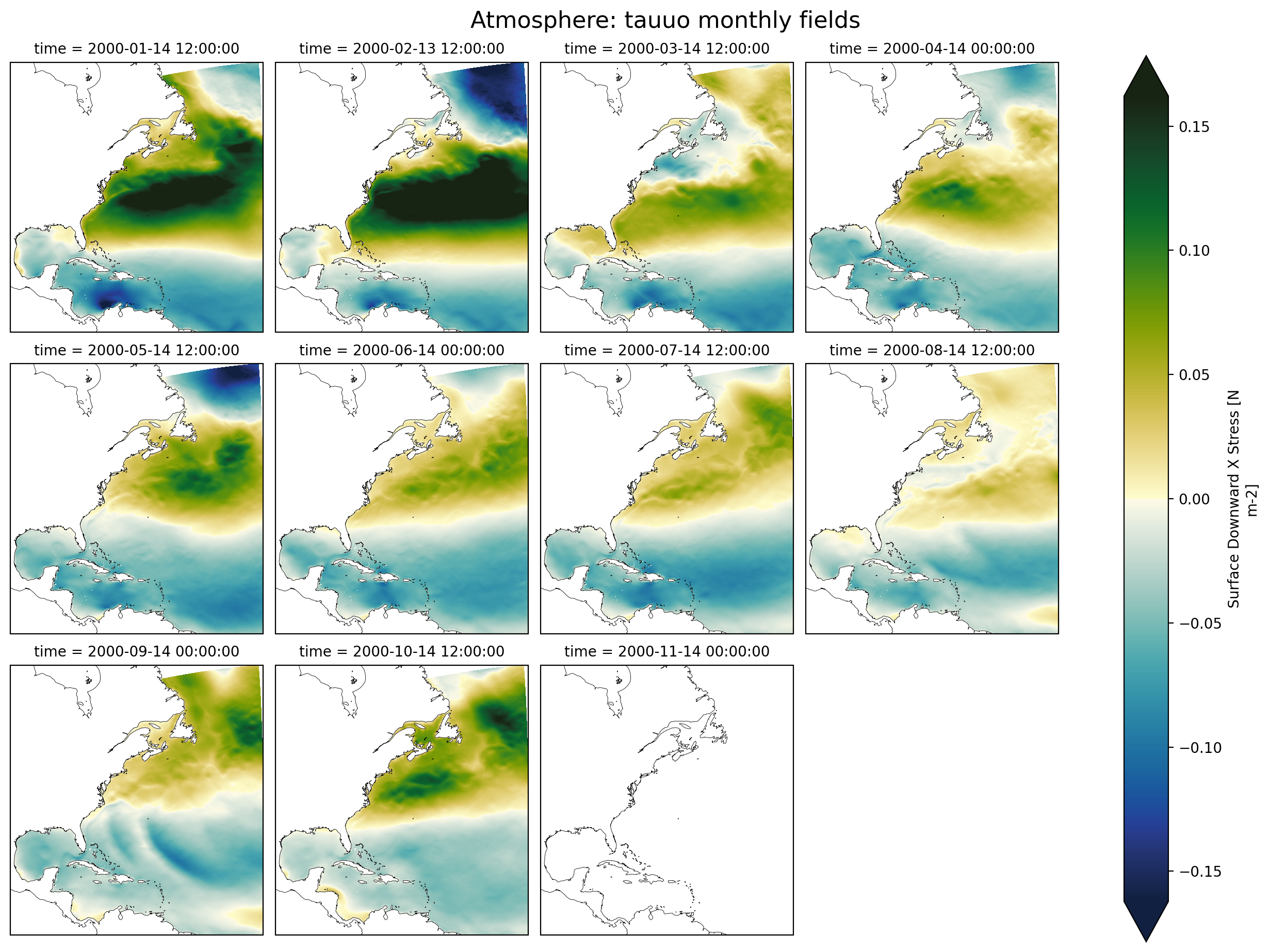
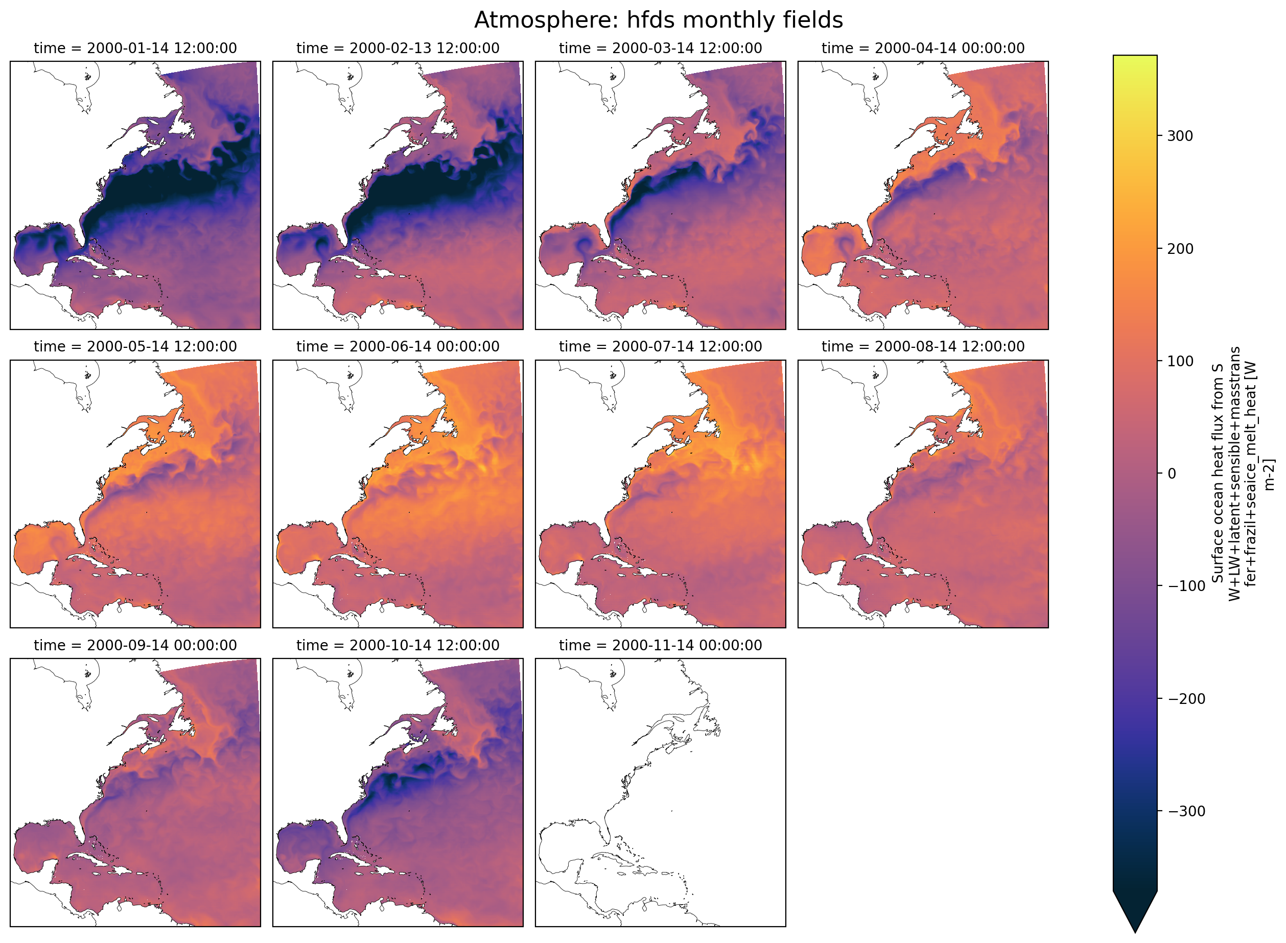
Simple Visualization of Atmospheric Forcing vs Ocean Variables¶

This notebook is short and sweet, designed to just show how we might access the atmospheric forcing variables. Pay particular attention to the meta data for the different variables!

Note: Native output can be weird, be wary and ask questions!

for coord in list(static_data.variables):
    if "geolon" in coord or "geolat" in coord:
        native_data = native_data.assign_coords({coord: static_data[coord]})
        monthly_data = monthly_data.assign_coords({coord: static_data[coord]})

for i, var in enumerate(atm_variables):
    field = native_data[var]
    sfc_var = ocn_variables[i]  # assuming order matches, it may not
    sfc_field = monthly_data[sfc_var].isel(z_l=0)

    geocoords = utils.chooseGeoCoords(field.dims)
    lon = geocoords["longitude"]
    lat = geocoords["latitude"]

    cmap = utils.chooseColorMap(var)

    transform = ccrs.PlateCarree()
    subplot_kwargs = {
        "projection": ccrs.Mercator(),
    }

    map_extent = [
        float(field[lon].min()),
        float(field[lon].max()),
        float(field[lat].min()),
        float(field[lat].max()),
    ]

    # Plot atmospheric variable for each month
    g1 = field.plot(
        x=lon,
        y=lat,
        col="time",
        col_wrap=4,
        robust=True,
        cmap=cmap,
        transform=transform,
        subplot_kws=subplot_kwargs,
    )
    plt.suptitle(f"Atmosphere: {var} monthly fields", fontsize=16, y=1.02)

    for ax in g1.axs.flat:
        ax.set_extent(map_extent, crs=ccrs.PlateCarree())
        ax.coastlines(resolution="50m", color="black", linewidth=0.3)

    if save_figs:
        plt.savefig(os.path.join(image_output_dir, f"{var}_monthly_grid.png"))
    plt.show()

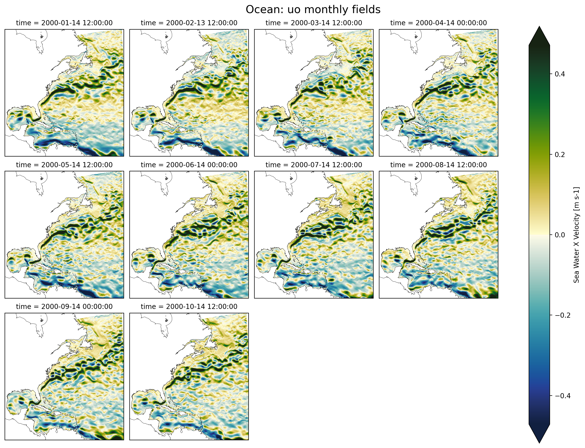
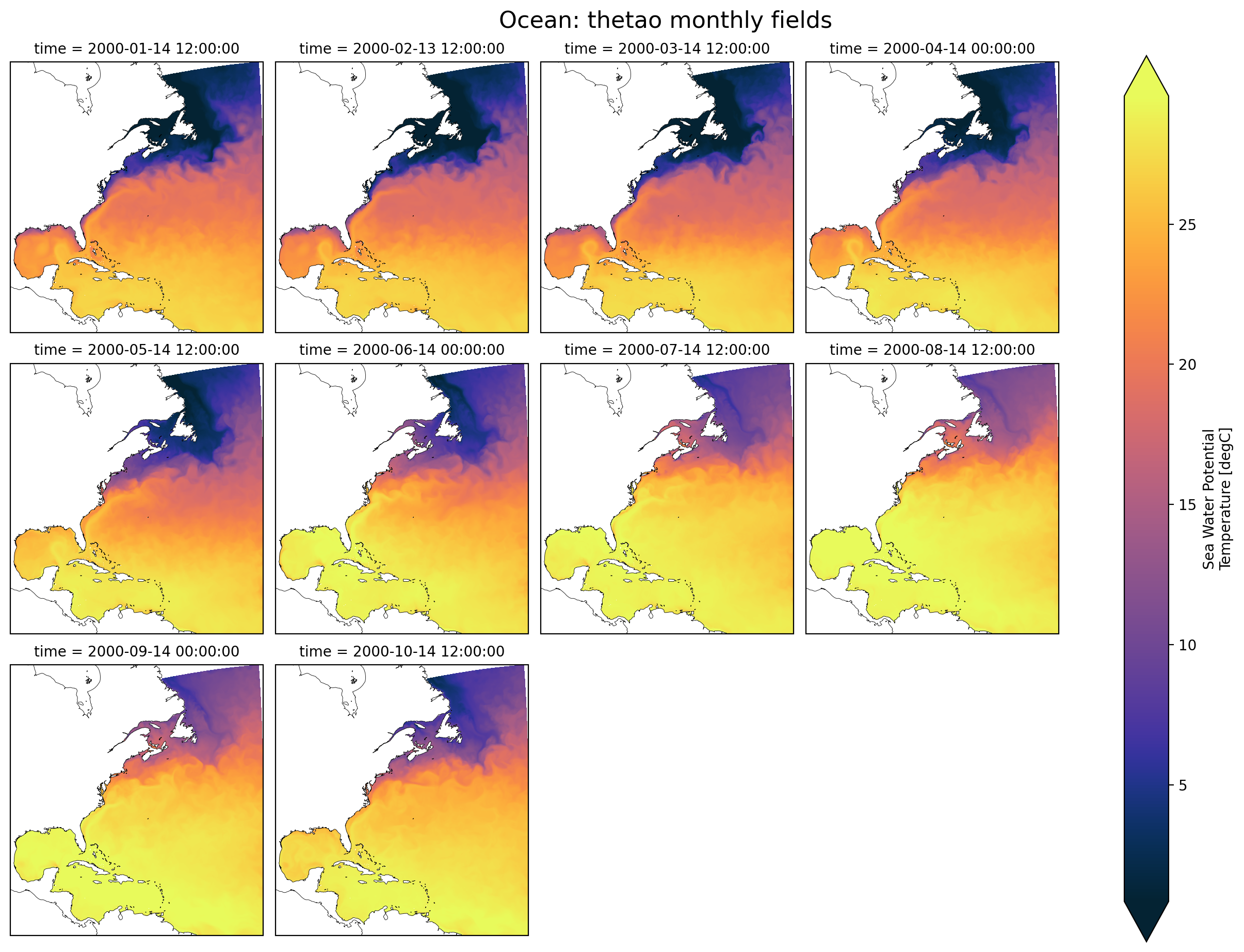
    # Plot ocean surface variable for each month
    g2 = sfc_field.plot(
        x=lon,
        y=lat,
        col="time",
        col_wrap=4,
        robust=True,
        cmap=cmap,
        transform=transform,
        subplot_kws=subplot_kwargs,
    )
    plt.suptitle(f"Ocean: {sfc_var} monthly fields", fontsize=16, y=1.02)

    for ax in g2.axs.flat:
        ax.set_extent(map_extent, crs=ccrs.PlateCarree())
        ax.coastlines(resolution="50m", color="black", linewidth=0.3)

    if save_figs:
        plt.savefig(os.path.join(image_output_dir, f"{sfc_var}_monthly_grid.png"))
    plt.show()